Summary
In this case, there is a necessity to analyze the results of the survey conducted for a commercial cleaning company. The purpose is to research the dependency between the quality of service and the number of worker hours spent in the customer’s facility. This paper will discuss a scatter plot created based on variables provided and a linear regression model to explain the variation and show the hypothesis test result.
Discussion of A Scatter Plot
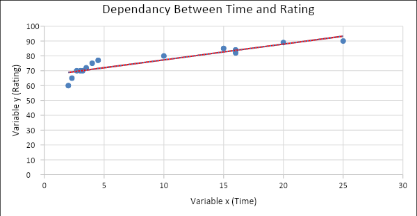
A scatter plot or scatter graph is one that utilizes dots to represent the values of different variables. There are two variables in this case: the rating of work and the number of hours spent. To begin with, it is necessary to decide which of the variables is dependent and which one is the independent one. Based on the rule that the independent variable is the cause, while the other one is an effect, it can be stated that they are time and rating, respectively. Therefore, in the chart, time (x – variable) is located on the horizontal axis while rating (y – variable) is on the vertical axis.
The tendency can be built using Excel’s tools to outline a dependency between the variables. As can be seen from Figure 1, the tendency tends to grow, which shows the positive correlation between the two variables (Yi, 2019). Therefore, the type of relationship is a positive one as well. The equation of the tendency is y = 1,0617x + 66,711. A Scatter plot is a valuable tool for providing a simple insight into dependency between two variables.

Discussion of a Linear Regression Model
The development of the linear regression model was done through a regression tool. There is the output that shall be considered to interpret the result. Multiple R amounted to approximately 0,915, which is a relatively high value, and as it is above zero, it indicates a positive and strong relationship between two variables, as well as the previously explained tool, does. The coefficient of Determination (R squared) value amounted to 0,83815, which implies that 83,8% of y-values are defined by x-values. The standard error amounts to 3.8%, which is a relatively small value that means that the result of the analysis has a considerable chance of being correct.
Then, analysis of variance (ANOVA) indicated the level of variability within the regression model. Significance F value equals 0,00000437, which is considered a low one as values greater than 0,05 suggest utilizing other predictors or show that the dependence between two variables is weak (Bevans, 2020). Residentials, or the differences between the observed values of the dependent variable and the predicted value, reveal that the outlined above equations, which are expected to predict the dependency between two variables, do not completely fulfill the function (Because, 2020). The part of the variability that the model explains is significant compared to the unexplained one, as the residentials that reflect the errors are relatively low and support the model’s strength.
In addition, P-value is much lower than the significance level, which supports the claim that there is strong relationship between variables, and the null hypothesis (that will be outlined further can be rejected). Despite the small number of observations that can make such an analysis’s results deceiving, all the examined indicators prove that the model is trustworthy, as the dependency is mostly explained, and the found relationship between variables is strong while also being a positive one according to the scatter plot.
Hypothesis Test
In this case, it is also possible to perform hypothesis testing. This method is used to determine the presence of a significant difference between the means of two groups (Mahesh, 2019). An alternative hypothesis for the future test is “rating depends on the working hours spent,” while the null hypothesis is “rating does not depend on the working hours spent. It is vital for the company to prove or refute the point that an increase in efforts results in an increase in rating. Therefore, the inverse dependency is not put emphasis on. It is vital to choose the appropriate T-test that would analyze the data correctly. Based on the same number of observations in both variables, an equal variance T-test is suitable (Mahesh, 2019). Simultaneously, based on the hypotheses, it is not significant to research how the increase in working hours spent can result in a lower rating as the inverse opinion is the priority. Thus, a one-tail equal variance T-test can be utilized.
According to the t-test, performed with consideration of the given significance level equals 0.10, there are the following results. Degrees of freedom or the number of valid observations equals 13. F value equals 0,744, which is higher than F critical, which amounted to (0,481). It implies that dependence cannot be proved, as means or variances are the same, so the variables are related to each other in the way they are expected to.
The null hypothesis can be rejected based on F values. However, based on a P one-tail value that equals 0,3, the null hypothesis cannot be rejected as the calculated value is much higher than the significance level (0,10). Despite confusing results, it is possible to make the following conclusions. The dependency between two variables, which are time and rating, is strong. Although the P one-tail value proves the opposite, all the other indicators show that it is possible to reject the null hypothesis.
References
Bevans, R. (2020). An introduction to simple linear regression. Scribbr. Web.
Mahesh, R. (2019). Everything You Need To Know About Hypothesis Testing – Part I. TowardsDataScience. Web.
Yi, M. (2019). A Complete Guide to Scatter Plots ChartI0. Web.