Summary
The viscosity of a fluid is associated with a quantitative indicator of a fluid’s tendency to resist flowing. It evaluates the fluid stress distribution caused by applied shear stress. Plane Couette flow is a primary fluid flow demonstration that illustrates the impacts of viscosity. The Couette flow depicts a fluid flow through two plates, one static and under constant stress. The top plate’s velocity is governed by fluid viscosity. The much more viscous liquid slower the vessels will travel.
Viscosity is a thermodynamics quantity changing as a function of temperature and pressure.The fluid viscosity often rises with pressure. The temperature may significantly impact the value of both the viscosity of a liquid. In gases, viscosity increases with temperature, owing to the increasing contact between gas molecules. The viscosity reduces with the temperature rise in fluids, owing to the more significant space between molecules. This characteristic is influenced by several variables such as physical properties of the molecules, molecule shape, and intramolecular forces, which are the forces of attraction here between molecules, the architecture of the fluid, and the temperature. The temperature is increased kinetic energy that overcomes the attraction forces; therefore, the molecules were able to flow past each other also freely and, as a consequence, produce less viscous liquid.
Purpose
- To measure and analyze the viscosities of perfect (toluene/p-xylene) and unstable (methoxy ethanol/water) two-fold solutions and their constituents.
- To investigate the impact of temperature variation on viscosity.
- To ascertain the activation energy associated with the viscous flow
Apparatus and Reagents
Apparatus
- Stopwatch
- Ostwald Viscometer
The Ostwald viscometer compares the flow duration of 2 liquids of known density. To use an Ostwald viscometer, fill the reservoir with liquid and suction it up to the top mark.
- Constant-Temperature Water Bath
- Burette
- Volumetric Flask
Reagents
- Toulene
- Distilled Water
- Xylene
- Methanol
Chemical Formulas
Mobile liquids are defined as having low viscosity. Fluidity is the inverse of density, F=1/. Non-associative liquid solutions are approximately additive, which is fluidity’s benefit. Because this experiment uses binary solutions, the mobility of a combination is provided by: Xa & Xb are the molar fractions. The mixture’s viscosity is given by: ln XA •A + XB •B 2) The second section of this lab measures viscosity-temperature dependency. A pure liquid’s viscosity increases exponentially. Viscosity is calculated using the flow rate of a liquid and its density. Equivalent viscosity, volume, and flow velocity of the standard liquid (water) are given in Equation 3.
Procedure
Suspend the viscometer in a 2-L beaker of water on a hot plate set to 25°C. Assemble the viscometer in the water.
- 20.00 ml of known density de-ionized water was Pipetted into the Ostwald viscometer and left to equilibrate to the bath’s temperature. Use a pipette bulb to raise the liquid level over the viscometer’s upper fiducial mark. As soon as the water returned to normal, the timer was started. And left until the meniscus hits the bottom point. The same procedure was repeated twice. The flow timings were between 0-4s.
- The viscometer was Cleansed and wiped using acetone. The acetone was cleaned and then aspirated for a minute to exhaust it.
- The flow rates of methanol/water mixtures were analyzed at 25°C
- the sequence was finished by measuring pure Methanol flow time. Repetition is required. These timings were within 0-4 seconds.
- As previously, the viscometer was carefully cleaned.
- As in step 3, the flow times of each toluene/p-xylene solution were changed. The experiments were then finished using pure p-xylene.
- The water bath was heated in 5 to 10-degree intervals for our temperature work, and the flow time of pure xylene was calculated as previously at each temperature. The temperature was kept constant. The precise temperature doesn’t matter as long as it’s within 0.5°C and the viscometer has already had time to adjust to the new temperature. At about 60° C, the practice was halted.
Data Analysis
The toluene combination was the perfect mixture, which had no hydrogen bonds or attractive forces. The non-ideal combination was methanol and water, owing to the sample’s attractive factors such as hydrophobic interaction components. This report also compared the experimental viscosity and fluidity to the predicted value to ensure both solutions were perfect. As the viscosity across both solutions falls, the answer is ideal. Last but not least, this report determined that as temperature rises, viscosity falls.
The solution flow may not have reached the capillary tube’s end, resulting in erroneous data, or the Ostwald viscometer may not have been fully submerged in the water bath, affecting the measurement temperatures.
This report plotted ln versus 1/T and calculated activation energy as the slope of a single direction. A line’s slope to make the figure linear, specific data points were discarded. Viscosities and therefore ln should decrease with temperature, but detailed data points defy this trend. This is due to timing problems and the inability to measure accurately at high temperatures.


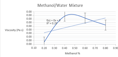
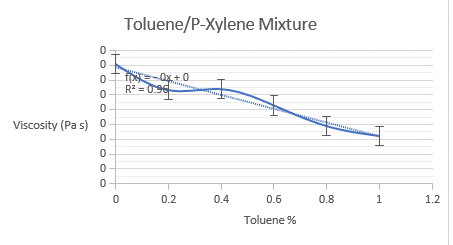
The viscosity of both binary mixtures was determined using the lab manual’s equation. Below are graphs of experimental and model-derived viscosities, including both binary mixes. The experimental viscosities estimated for methanol/water combination do not follow a linear trend, perhaps due to experimental/human error. The measured viscosities for toluene/p-xylene mixes follow a linear trend, as predicted by the equation.
The ideality of both the water-acetone & toluene-xylene systems were determined using theoretical and experimental fluidities. Theoretical fluidities were calculated using inverse viscosities of pure solvents. The discrepancies between theoretically and experimentally fluidities were used to conclude the systems’ ideality. As can be observed, pure water has more significant relative viscosity coefficients than acetone. Strong hydrogen bonds form between water molecules but not acetone molecules.
Strong dipole-dipole interactions between water and acetone molecules explain high coefficients of viscosity. The relative variable of viscosity decreases with increasing temperature. As previously stated, the toluene-xylene system has weak van der Waals forces. The low coefficients of viscosity reinforce this. Intermolecular forces among xylene molecules are more significant than intermolecular interactions between toluene molecules. Theoretical and actual water-acetone fluidities differ significantly, whereas toluene-xylene fluidities are almost identical. The toluene-xylene system may be considered to be perfect.
So intermolecular interactions between toluene and xylene molecules are almost identical to intermolecular interactions in a combination of these solvents. However, intermolecular interactions in pure water and acetone are distinct from those in the water supply. Water is the only one of the four solvents that possess hydrogen bonding. Water and acetone both have dipole-dipole interactions. Dispersion forces exist between molecules in all liquids, although xylene contains one more carbon than toluene. The ignition energy is directly linked to the molecular interactions of contacts. The intensity of the experimentally measured activation energy rises as follows: toluene xylene water Acetone’s activation energy was predicted to be greater than xylene’s and lower than water. The acetone activation energy does not corroborate the trend. This may be due to measurement mistakes.
Reference
Exp.3: Viscosity of Liquids, Part I.