Introduction
The study was done in 2015 and involved a sample of 486 students aged 18- 25 years from across 40 universities in the United Kingdom. The study aimed at investigating the predictors of young drinking behavior. The variables from the study include age, sex, alcohol, dn, int, ssimp, inj, and swl. Alcohol has been a problem among University students where some studies have shown high alcoholism rates to be as high as 85% and female students drinking as much as males (Davoren et al.). The paper will use parametric methods to infer the predictive power of the various variables to drinking intention. The first parametric method is correlation analysis followed by multiple regression. Hierarchical multiple regression is used to check the incremental power of adding specific variables at a time.
Methods
The participants of the study were university students from 40 different universities across the United Kingdom. The total number of participants was 486 aged between 18 and 25; the age with the highest frequency was 20 with 107 measurements, while the least was 25 with 20 observations. Out of all the students, there were 101males and 385 females. The primary variable of the study is drinking intention among the participants. The variables inj, ssimp, swl, and dn were measured on a 7-point Likert item with a Cronbach’s reliability alpha also being run.
Results
Descriptive Statistics

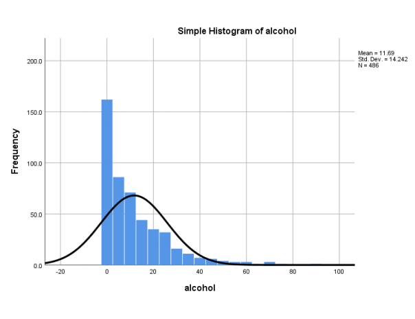
From the figure above, the data is not symmetrical and is skewed to the right. The peak of the normal curve does not coincide with the distribution’s maximum frequency. The distribution of alcohol is not normal. The variable also has a minimum value of 0, a maximum value of 91, and a mean of 11.69.

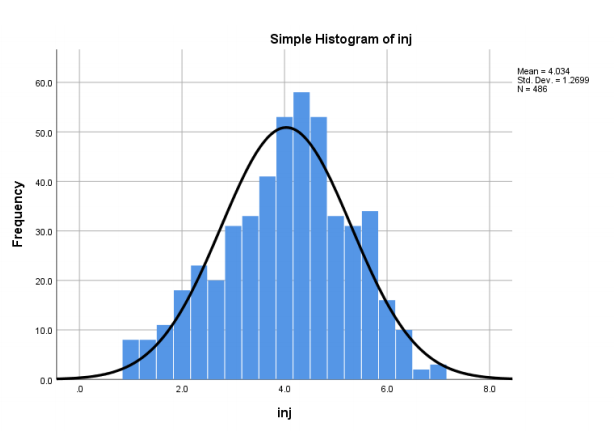
The above figure represents a histogram and a normal curve for inj. The normal curve seems to follow a normal distribution or within acceptable limits of normal distribution because the normal distribution curve’s peak coincides with the highest frequency values (Hopkins et al., 2018). The mean and median seem to also be concentrated at the center. The variable passes the eye-test for normal distribution.

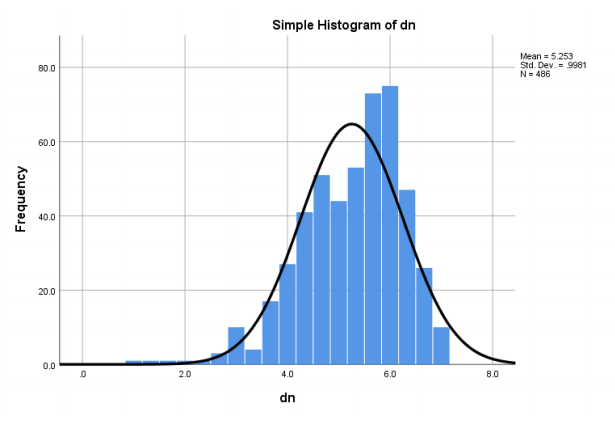
The third variable, dn, seems to have a slight skewness to the left. The mean of the sample is 5.25, which is close to the points with maximum frequency. Although the normal curve’s peak does not coincide with the peak of the histogram, the difference is not too significant to rule out a normal distribution. The variable, therefore, passes the visual test for normality. The mean for age was 20.46, while the standard deviation was 1.82.
The mean for alcohol was 11.69, while the standard deviation was 12.24. The variable inj had a mean of 4.03 and a standard deviation of 1.27. On the other hand, ssimp had a mean of 4.4 and a standard deviation of 1.2; there were 9 missing values for ssimp. The variable swl had a mean of 4.15 and a standard deviation of 1.37; there were 3 missing values for swl. On the other hand, dn had a mean of 5.23 and a standard deviation of 0.998. for the variable int, the mean was 4.6, and the standard deviation was 1.80.
Correlation
The Pearson correlation coefficient test was carried out on the variables age, sex, alcohol, inj, simp, dn, and int to check how the different variables correlated. The SPSS results gave results of Pearson correlation coefficient and significance score for each variable pair. For two variables to be significantly correlated, the significance value was larger than the considered alpha values. In this case, the following were the results: Age and inj had a low negative correlation with r(484) = -0.092, p = 0.042. Age and dn had a low negative correlation with r(484) = -0.097, p = 0.032. Sex and alcohol had a negative low correlation where, r(484) = -0.112, p = 0.014. Alcohol and inj were found to have a low positive correlation r(484) = 0.199, p = 0.00. Inj and ssimp had a low to moderate positive correlation with r(484) = 0.286, p < 0.001.
Alcohol and dn were also found to have a low to moderate correlation with r(484) = 0.253, p < 0.001. Alcohol and int had a moderate positive correlation with r(484) = 0.417, p < 0.001. similarly, inj and dn were also found to have a moderate positive correlation where, r(484) = 0.418, p = 0.00. Moreover, int and inj had a low to moderate positive correlation where r(484) = 0.24, p < 0.001. Swl and simp were found to have a low positive correlation where r(484) = 0.167, p < 0.001. On the other hand, dn and int had a low to moderate positive correlation where r(484) = 0.279, p < 0.001. Int and ssimp had a low positive correlation where r(484) = 0.228, p < 0.001. From the correlation results, the largest absolute value for correlation was 0.417 which is just moderate.
Regression
The first regression was planned with int as the dependent variable and dn, swl, ssimp, and inj as the regressors. Multiple regression is performed with the assumption of independent observations, normality, homoscedasticity, and linearity. Visual inspections were used to check for these assumptions. The independent variables test was inferred from the assumption that the study was carried out from students who had not interacted in a way that would influence their answers.
PP plots and histograms were used to check for normality. From the PP plots, it was discovered that all the variables met the conditions for normality assumption since all the points fell along the 45-degree line. Since they were not time series data, autocorrelation was not a concern. It was also important to keep in mind that the samples were also quite large, which bolstered the normality assumption. With the tests out of the way, the multiple regression was carried out as shown in the table below.
Table 2. Regression Coefficients for Predicting int from dn, swl, ssimp, and inj.
The first regression test was carried out with int as the dependent variable and dn, swl, ssimp, and inj as the predictor variables. The multiple linear regression results indicated a significant collective effect between int, ssimp, swl, and dn. (F(4, 469) = 20.68, p <.001, R2adj =.143). The individual predictors were examined further and indicated that ssimp (t = 4.987, p <.01) and dn(t = 4.253, p <.01) were significant predictors in the model.
The second regression model is the hierarchical type where a variable is tried at first with a section of variables then with another set of variables. In this case, the first set was alcohol, age and sex. This model was significant with the independent variables explaining 17.6% variability in int. After adding swl, inj, ssimp and dn, there was an R-square change of 0.065. This means that all the other variables added a 6.5% of predictive power to the first model. The summary of the first model was F(3, 470)= 34.76, p<0.01, R2adj =.176. The summary of the second incremented model was F-change (4, 466) = 9.97, p<0.01, R2adj change =.065.
The third regression model analyzed was also a hierarchical one with int still the dependent variable; for this experiment, sex=female. The first block of variables was alcohol and age; the second block added swl, inj, ssimp, and dn. The first block of independent variables explained 21.4% of the dependent variable, while the second block explained an additional 7.2%. The first model’s summary is F (2, 97) = 14.45, p < 0.01, R2adj =.23. The second model’s summary was F-change (4, 93) = 0.072, p=0.057, R2change=.072. From the data, the second model was not significant. When this same regression was repeated with sex=female, the summary was F (2, 371) = 38.79, p<0.01, R2adj =.173 for the first model and F-change (4, 367) = 7.533, p<0.01, R2change =.063. The coefficients tables showed that age was insignificant in the first block of variables, while in the second block, inj and age were insignificant.
Discussion
The analysis showed that different factors combined could be used to predict drinking intention at different rates. The model with the highest prediction capacity judging by the R2adj was the model where the adjusted R square was 25.6. This model’s independent variables were age, alcohol, ssimp, inj, swl, and dn. For this model, however, only alcohol and dn were significant. For almost all models, sex and age were not significant variables to predict the intention to drink. This finding is consistent with the literature review that showed that girls are drinking as much as boys.
Interestingly, age was also an insignificant variable in predicting intention to drink; it is counter-intuitive since one would expect first-year students to be timid and refuse to drink. The reason why age did not matter is probably that the younger the student, the more likely they lacked drink refusal self-adequacy. The study concludes that the intention to drink is mainly predicted by the variables dn and alcohol since they predicted the dependent variable’s variability the most. It is no surprise that sex was shown to be insignificant backing literature review about closing gender gap in drinking behavior.
Reference
Davoren, Martin P., et al. “Alcohol Consumption among University Students in Ireland and the United Kingdom from 2002 to 2014: A Systematic Review.” BMC Public Health, vol. 16, no. 1. 2016, p. 173. Web.
Hopkins, S., Dettori, J. R., & Chapman, J. R. (2018). Parametric and nonparametric tests in spine research: Why do they matter? Global Spine Journal, 8(6), 652–654. Web.