Introduction
There are any number of real-life, pragmatic reasons for studying the behaviour of electricity markets. While this paper revolves on a database from the 1937-1938 period in UK history, when voluntary compliance by regional power monopolies with a central electricity authority was the rule, contemporary circumstances predicate even more watchful analysis.
For instance, contemporary concerns about global warming and the ‘carbon footprint’ of the UK power industry (accounting for half of all emissions in the UK) virtually dictate official attention to matters of fuel in use and the national volume of electricity consumption.
Secondly, the advent of spot markets even for electricity has required even greater vigilance and sophistication about day-ahead forecasting performance of price models that account for the impact of economic, technical, strategic and risk factors on even intra-day prices, and how these effects behave over time. Addressing these concerns, Karakatsani and Bunn (2008) found that models relying on market fundamentals and time-varying coefficients have the best predictive performance of all alternatives when applied to the British market.
Methodology
Develop a multiple regression model which could be used to predict the demand for electricity (KWH) from all the other variables in the database: CUST, INC, MC4, MC6, MC8, GAS6, GAS8, CAP AND EXPEN. The variable definitions are as follows:
- CUST Average number of consumers with two-part tariffs in 1937-38, in thousands;
- INC Average income of two-part consumers, in pounds per year;
- MC4 The running charge (marginal cost) on domestic two-part tariffs in 1933-34, in pence per KWH;
- MC6 The running charge (marginal cost) on domestic two-part tariffs in 1935-36, in pence per KWH;
- MC8 The running charge (marginal cost) on domestic two-part tariffs in 1937-38, in pence per KWH;
- GAS6 The marginal price of gas in 1935-36, in pence per therm;
- GAS8 The marginal price of gas in 1937-38, in pence per therm;
- KWH Consumption on domestic two-part tariffs per consumer in 1937-38, in kilowatt hours;
- CAP The average holdings (capacity) of heavy electric equipment bought on hire purchase (leased) by domestic two-part consumers in 1937-38, in kilowatts;
- EXPEN The average total expenditure on electricity by two-part consumers in 1937-38, in pounds.
The database to be tested contained 42 observations or cases.
The reference here to two-part electricity tariffs is to the Act of 1926, which established a public interest corporation, the Central Electricity Board (CEB). The CEB was mandated to, among others, construct a national transmission grid and rationalize UK electricity prices (Foreman-Peck and Hammond, 1997). During the era represented by the database, public utility monopolies in the Kingdom usually raised revenue through a two-part tariff consisting of a standing charge (or ‘line rental’), which must be paid to gain access to the utility; and a price for each unit consumed (or running rate, Salies and Price, 2003). The existence of three different unit prices, denoted MC#, in the database reveals the existence of electricity price increases approved by the CEB between 1933 and 1938 (see variable definitions above).
The power generation industry was privatised in the eighties and nineties but reregulated in recent years. A dual-tariff structure remains in effect, albeit varying by region across the UK.
In Minitab 15, load data file ‘UKELEC.MPJ”. Then trigger, in succession, the command sequences for:
- Scatter plots of all the (presumed) predictor variables against the criterion variable KWH by executing Graph-Scatterplot, in order to winnow out the candidates for the next step.
- Quantify the nature of the relationship between KWH and each predictor variable by performing simple correlation and linear regression (Stat-Basic Statistics-Correlation.
- Test the ability to predict KWH from the meaningful combination of predictor variables with a multiple regression run: Stat-Regression-Regression. In the menu, type in, or transfer ‘KWH’ to the ‘Response’ box. Tab to ‘Predictors’ and choose (or type in) the assigned predictor variables: CUST, INC, MC4, MC6, MC8, GAS6, GAS8, CAP AND EXPEN.
Choose all necessary diagnostic options in the sub-menus.
Findings
One-to-One Relationships
The first screen on the database reveals that several variables are inversely correlated with electricity demand. These are CUST, MC4, MC6, MC8 and GAS8.
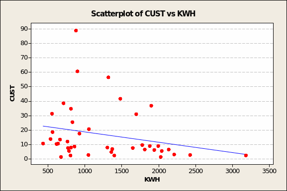
For CUST (see Figure 1 overleaf), the inverse nature of the relationship looks to be unusually affected by the extreme value of the outlier pair with a CUST value of 2.2 but KWH consumption of 3,183 (see lower right quadrant of chart). There are other outliers in the upper left quadrant (e.g. KWH demand = 874, CUST value = 88.7; KWH demand = 896, CUST value = 60.6; KWH demand = 1,314, CUST value = 56.4; and three others closer to the calculated trend line) but without the first-mentioned extreme value, their likely effect is to provoke a flat demand curve.
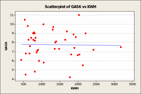
Such a flat demand curve is demonstrated by the plotting the intersections of GAS6 and electricity demand (Figure 2 overleaf). Both the data scatter and the flat trend line bode no good for hypothesizing any meaningful relationship between whatever GAS6 represents and electricity demand in the UK.
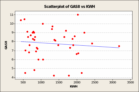
Like CUST, GAS8 appears inversely correlated with KWH (see Figure 3 overleaf). In an otherwise random scatter of pair-points, an extreme case like that at the rightmost edge (KWH demand = 3,183, GAS8 value = 7.5) can tug the trend line downward, as do the outliers in the bottom-middle area.
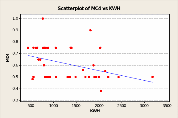
MC4, which varies within a very narrow range of 0.4 to 1.0, also evinces an inverse relationship with electricity demand (Figure 4 below). This time, it is the influence of ‘upward-tugging’ outliers in the upper right quadrant (low KWH demand = 758, MC4 value = 1.0; modest KWH demand = 1,811, MC4 value = 0.9) that alter what is very likely a flat trend line. In short, the correlation value is likely to be close to zero.
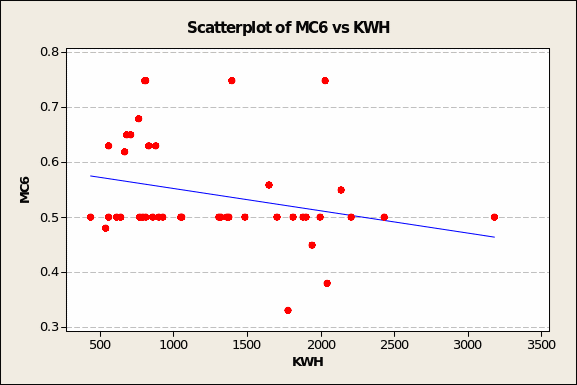
Very much the same ‘anomaly’ seems to characterise the association between MC6 and electricity demand (see Figure 5 overleaf). What should clearly have been either flat or gently sloping downward is unduly influenced by outliers in the upper right quadrant (low KWH demand = 798, high MC6 value = 0.75) and the lower middle third of the chart (e.g. moderate KWH demand = 772, low MC6 value = 0.33).
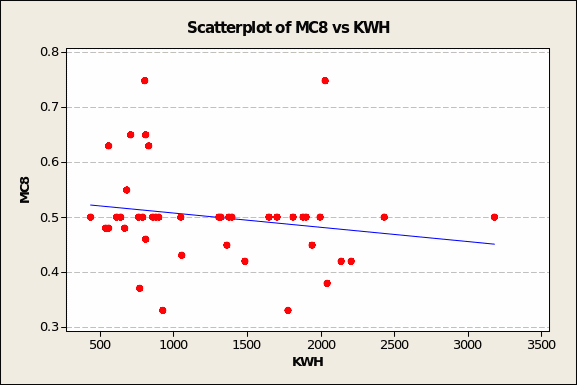
Similarly, the semblance of an inverse relationship between MC8 and KWH (see Figure 6 overleaf) has to be carefully evaluated owing to upper-left quadrant (e.g. low KWH demand = 798, high MC8 value = 0.75) and lower middle third (e.g. moderate KWH demand = 1,772, very low MC8 value = 0.33) outliers
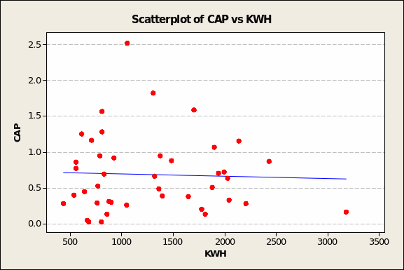
Like that for GAS6, the relationship between CAP and electricity demand should display as flat or random except for the opposing pull of outliers in the upper left (low KWH demand = 1,052, maximum CAP value = 2.52) and lower right (very high KWH demand = 3,183, very low CAP value = 0.17) quadrants. As a result, the relationship looks to be inverse.
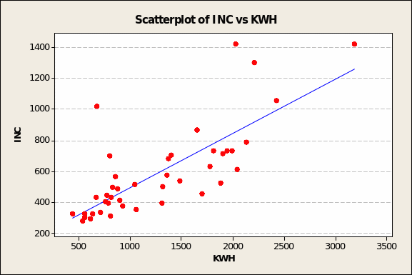
On the other hand, the predictor variables that may be of interest for correlation tests and inclusion in a predictive model – by reason of showing even a slightly positive and linear relationship – are EXPEN and INC (see Figures 8 and 9 overleaf).
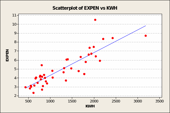
The results of multiple correlation analyses confirm what visual inspection deduced from the scatter plots: electricity demand is most closely related to average total expenditure on electricity by two-part consumers in 1937-38, in pounds (EXPEN, Pearson’s r = 0.87) and to average income of two-part consumers, in pounds per year (INC, Pearson’s r = 0.77). In both cases, Minitab returned p values lower than 0.005. This means that the twin conclusion about INC and EXPEN being closely related to KWH has less than 5 chances in 1,000 sampling tries (of UK households) of being wrong.
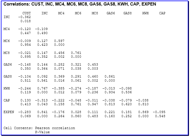
Income as a predictor variable aside, one must view with caution the the finding that EXPEN correlates highly with KWH. Since the former represents payments to the utility while the latter is about unit consumption, the prudent analyst should be watchful for collinearity.
Linear Regression and the Derived Multiple Regression Model
Testing, first of all, for the simple linear regression between INC and KWH, we obtain the following result and diagnostics:
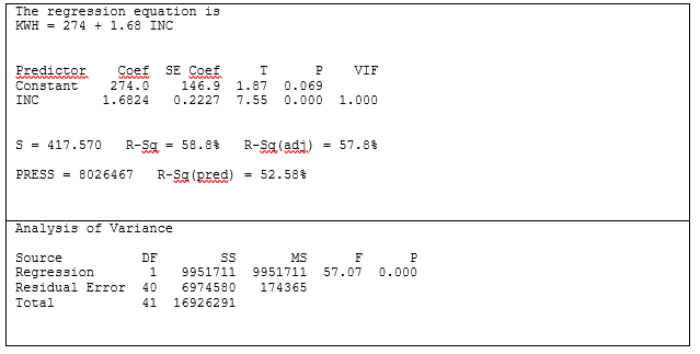
This is the mathematical expression of the relationship graphed in Figure 9 (page 8) where, first of all, the intercept is at 274 KWH. This is tantamount to the minimum level of electricity consumption when neither income nor any of the other predictor variables are accounted for. In statistical terms, this is the likely KWH consumption when income is zero. In the real world, of course, income is never zero.
Further, the value of the coefficient β = 1.6824 suggests that electricity consumption rises by 1.7 KWH for every £1 gain in annual family income. In short, electricity use increases disproportionately with income.
At p < 0.005, such a relationship between INC and KWH is likely to hold in 995 out of a thousand samplings of UK households. The odds are very low that such a result could have occurred by chance alone.
While the ANOVA portion of the linear regression model yields such a high F value as to preclude pure chance (p <0.005), the proportion of the variance in the criterion variable accounted for by income (R2) is robust enough at 58% to suggest that INC will prove to be the primary predictor variable when multiple regression model is built.
Constructing this model, we select INC and other predictor variables that attained satisfactory correlation with KWH in Table 1 (page 9). These are EXPEN and the three MC# variables (CUST must be set aside because it accounts for population size whereas the criterion variable, KWH, is expressed in per-capita consumption terms).
The first component of this prediction model, though the least important, is the initial number on the right hand side of the equation, 1134.7. This is technically known as the “intercept”, the starting point for the prediction line if one were to chart the result of the prediction model. It is a value on the Y axis, meaning that over the time period for which there is data, annual electricity consumption amounts to 1,135 KWH (see also the first value Minitab reports in the ‘Coef’ column above, Table 3) if none of the independent variables were in effect. In short, one may consider the intercept as something akin to a ‘base value’ in this analysis.
The second point worth noting is that the prediction model contains a mix of plus and minus signs. This combination reveals that electricity consumption is directly proportional to family income and average spending on electricity (keeping in mind the earlier caveat about autocorrelation) but inversely proportional to all the marginal or running charges in the two-part tariff structure that prevailed from 1933 to 1938.
And the third, most important piece of information is embodied by the ‘beta coefficients’, the values associated with each predictor variable. These tell us that, taken together:
- An increase of £0.48 in average annual family income will lead to an increase of 1 KWH in the criterion variable.
- Similarly (again, this must be treated cautiously), an increase of £236 in average electricity payments through 1937 and 1938 should boost electricity demand by 1 KWH. The workings of collinearity are obviously at work here since power could not possibly have cost so much in the pre-war years.
- In turn, the composite index is inversely related to marginal costs on domestic two-part tariffs. Specifically, an increase of 880 pence per KWH in 1937-38 tariffs, 338 pence per KWH in 1933-34 tariffs and 1242 pence per KWH in 1935-36 tariffs depresses electricity consumption by one KWH.
What the above show is that electricity consumption was both income- and price-elastic.
Diagnostics
How well does this predictive model stand up to the standard indices of reliability and explanatory power?
First of all, there is R, the correlation between the observed value and the predicted value of the criterion variable. The computed value for Pearson’s R (0.93) shows a near-optimal fit between the actual and predicted levels of the composite index.
R Square (R2), shown in the Minitab model summary (Table 4 ), is the square of R and reveals the proportion of the variance in the criterion variable accounted for by all four variables incorporated in the model. Thus, INC, EXP, MC4, MC6 and MC8 together account for a high 87% of the variance in electricity consumption.
R2 is a fundamental and widely-cited measure of how good the prediction of the KWH criterion variable becomes as long as we have reliable information on where the predictor variables are headed.

However, R2 is prone to slightly over-estimate the success of the model when applied to ‘real-world’ rigour (Gujarati, 1999). Hence, Minitab also calculates an ‘Adjusted R2 value to account for the number of variables in the model and the number of observations (probably regions in the UK, in this case) the model is based on. At 85.2%, the Adjusted R2 value renders the more reliable measure of the success of the model. In this case, we are more confident that the model has accounted for 85% of the variance in the criterion variable. This measure of the strength of the relationship between actual power consumption and the predicted KWH is called ‘multiple correlation’.
Given the beta coefficients and the standard error for each, we can derive the 95% confidence interval via: β ± (1.96*SE). Following this, we derive the intervals below with only a 5% chance that we are wrong:
- INC = -0.01042 to 0.96762
- EXP = 159.742 to 311.838
- MC4 = -1039.18 to 364.18
- MC6 = -2622.232 to 138.232
- MC8 = -2201.436 to 441.036
By way of example, we state that every additional pound sterling in annual family income either reduces KWH by 0.01 throughout 1937 to 1938 or adds 1 KWH.
We then need to address a second major concern in model diagnostics, parsimony. That is, does the predictive analysis include as few predictor variables as possible by eliminating those that are highly correlated with each other? This is known as testing for collinearity.
The concern with collinearity springs from the intercorrelation findings (Table 1 in page 9) that MC4, MC6 and MC8 all bear correlations with each other of at least 0.456. As well, EXPEN is highly correlated with KWH.
Other measures for detection of multicollinearity, as suggested by Gujarati (1999, 322) are:
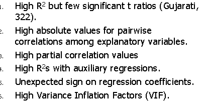
If none of the 6 items are detected, there should not be any multicollinearity in the model. But multicollinearity is a strong supposition if at least one of the 6 items is found.
For the first test, Table 3 (page 11) affirms that R2 is high (85% of variance explained) but all the t ratios except for EXPEN fail the statistical significance hurdle of α = 0.05.
On the other hand, the model meets the test of ‘High partial correlation values: abs(pcv ) > 0.9’. All the partial correlation values in Table 1 turn out to have absolute values ranging from 0.19 to 0.87.
Thirdly, all the Variance Inflation Factors (VIF’s, see Table 3 above) except for MC4 are greater than 2.
Table 5.
One therefore concludes that the model contains multicollinearity. Refining the model to eliminate these will require eliminating at least one of the predictive variable (EXPEN, most likely, since it is the pounds expression of the criterion variable KWH) or re-sampling from more recent periods, reconceptualise the model, restudy the literature to gain new insight on other predictor variables, or transform the variables (Gujarati, 331-334).
Continuing with diagnostics for this regression model, we see from the Analysis of Variance section of the output that at 5 degrees of freedom, the computed F value is 48.2 (see Table 6 below). An F value of this magnitude can occur by chance less than five times in a thousand sampling runs of regional electricity markets in the UK. Hence, we conclude that the model permits predictions of extremely high confidence.

Yet a sixth diagnostic available in the multiple regression model is the Durbin- Watson test, employed to test the hypothesis that the autocorrelation parameter, r, is zero. Specifically…


For the number of predictor variables k = 5 and n observations = 42 (~40 in Savin and White, 1977), the standard table for the Durbin-Watson Statistic at 5 Per Cent Significance Points of dL and dU provides hurdle values of 1.047 and 1.583 for dL and dU, respectively. Since the calculated Durbin-Watson statistic = 2.10172 is higher than the dU value, we conclude that the autocorrelation coefficient is not present and accept the null hypothesis. There is no autocorrelation in this database: consumers in UK regions consume electricity irrespective of prior states of the market.
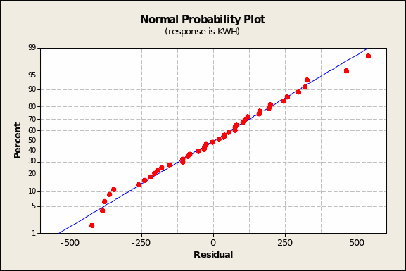
Lastly, one checks the model based on the ‘four-in-one charting’ facility available in Minitab. Were the residuals normally distributed, the Probability Plot of the KWH predictor variable should show all the red (predicted KWH) points very close to the blue line and an overall shape resembling a normal distribution. This is the case (Figure 10 below).
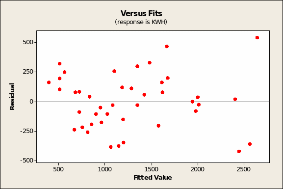
The residuals versus fitted values (Figure 11 overleaf) shows, as expected, random scatter. On the other hand, the model is rendered somewhat weak by the finding that the histogram of residuals (Figure 13 overleaf) does not quite show a normal distribution.
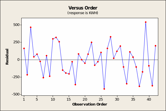
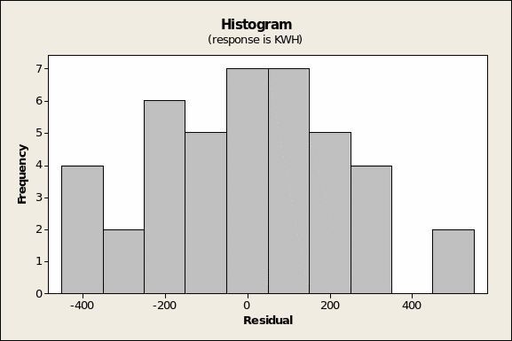
In turn, the observation order chart (Figure 12 in prior page) is a critical diagnostic only if the order of observations in the dataset has some meaning. This does not seem to be the case for the electricity database.
Conclusions
It stands to reason, of course, that family incomes are a very strong predictor of electricity consumption. The upper class – represented in 1937 and 1938 by households earning from £800 to in excess of £1,400 a year – are bound to demonstrate the phenomenon of rising expectations. That is, the more one makes, the higher the lifestyle one aspires for, quite irrespective of aspirations handed down from centuries of hobnobbing with the aristocracy and peerage. Even in this day and age, being well-off can still mean having a country seat and a larger residence in town. More homes mean more servants, more electrical conveniences (as evidenced and disproportionately high per-capita electricity consumption.
Recommendations
The results of this analysis have implications beyond the purely academic. In an age when governments must concern themselves with the environmental costs of electricity generation – Salies and Price (2003) report that the sector is responsible for half the carbon dioxide emissions in the country – efforts to comply with the Kyoto Protocol for emissions reduction may well extend to restructuring tariffs so as to combat the income-elasticity of electricity consumption. This likely entails at least a three-rate structure that charges families consuming more than 1,000 KWH disproportionately more and thereby signals to the public at large that the convenience of electricity comes with enormous social costs.
Bibliography
Foreman-Peck, J. S. & Hammond, C. J. (1997) Variable costs and the visible hand: The re-regulation of electricity supply, 1932-37. Economica, 64, no. 253, pp. 15-30.
Gujarati, D. (1999) Essentials of Econometrics. 2nd ed. Boston, Irwin/McGraw-Hill.
Karakatsani, N. V. & Bunn, D. W. (2008) Forecasting electricity prices: The impact of fundamentals and time-varying coefficients. International Journal of Forecasting. Vol. 24, (4) pp. 764-785.
Salies, E. & Price, C. W. (2003) Pricing structures in the deregulated UK electricity market. Discussion Paper, Department of Economics, School of Social Sciences, City University London.
Savin, N.E. & White, K. J. (1977) The Durbin-Watson Test for serial correlation with extreme sample sizes or many regressors. Econometrica 45, pp. 1989-1996.