Classical Macroeconomic Analysis and Its Principles Research Paper

Classical Macroeconomic Analysis

In this chapter, the book focuses on classical macroeconomic analysis as it was before the Great depression, which greatly revolutionized macroeconomic analysis as we know it today: bringing forth fiscal policy measures and the advantages therein, such as economic recovery. According to classical macroeconomic, money supply did not respond to changes in interest rates during the early 1900s because of:

1. the gold standard, that is the standard economic unit of account is a fixed mass of gold (held by the treasury),
2. the concept of finance companies (as a sector) lending money, was still relatively new.

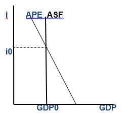
Due to the fact that classical macroeconomists had not factored in variables such as corporate lenders, investment of idle cash from sales by giant private firms and investment of temporarily idle taxes by government, which normally cause the money demand (M) and Velocity of money (V) to respond to interest rate changes, the Aggregate Supply of Funding (ASF) line was plotted vertically. Further, the classical economists had not come up with a hypothesis pertaining to how the Aggregate Planned Expenditure (APE) responds to changes in Gross Domestic Income (GDY) therefore, their diagrams lacked an IS line (which is present in modern day diagrams).

The APE line, where the economy is in equilibrium (from a classical macroeconomist’s point of view) is similar to a present day diagram. As illustrated in the diagram, where GDP=APE=ASF (Io and GDP0), ASF line however being atop the GDP line.

The repercussion of the ASF line being horizontal is seen given a scenario where the APE line shifts to the right (at the existing interest rate levels); implying an increase in expenditure with no funding to compliment it. Meaning, due to the unresponsiveness of M and V to changes in the interest rates, the rates just continue to rise but the funding doesn’t increase. Firms end up not bothering with increases prices or output because the demand that would have been there has been crowded out by very high interest rates.

In a scenario where expenditure reduces, funding becomes excess and those who hold it (in a desperate bid to find borrowers) give it out at gradually lower interest rates. All these scenarios come into play because the classical macroeconomists did not factor in certain assumptions, for example, firms would ultimately have to go out to borrow to pay for accruing inventory before sales bounce back.

In as much as the ASF line is vertical, in the event that it is detached from the GDP and APE, the following observations are made: In a scenario where there is excess funding in the economy (ASF line shifting to the right), such that ASF is more than GDP (at interest level Io), prices will be increased by firms because the level of funded demand exceeds output. Classical economists assume that firms will be operating at profit-maximization levels. The ripple effect continues until interest rates, ASF and APE return to their original points. The vice-versa is also true where ASF drops and a decrease in prices is observed. It should however be noted that employment and levels of output remain unchanged.

With respect to GDP, similar inferences are made where its drop would pull the funding and expenditure down with it due to the fact that prices and interest rates would increase. In the event that GDP rose, the opposite would be observed, where prices and interest rates would behave in the opposite direction to create a scenario where ASF and APE strive to adjust to be on the same level as GDP.

Duly noted, until the Great Depression came, employment and output were unaffected.

The Federal Reserve System

The Federal Reserve System (Fed) came into being in 1913, courtesy of Congress, as a result of some predicaments plaguing the financial sector beginning from early 1900s. The Fed was an idea suggested by the National Monetary Commission (which was also formed by congress), delegated the duty of stabilizing the economy through management of the nation’s money supply and control of the banking system, which if not carried out effectively and efficiently would see it dissolved/altered by the congress (despite the fact that it was independent of the congress).

Federal Reserve Banks were formed and are run by the federal government and in as much as most are not part of Fed; all have to comply with its regulations. Fed’s revenue caters for its operational costs, dividends for shareholders, emergency fund and financing programs (of the federal government).

The Fed’s Board of Governors, together with the Federal Open Market Committee are required by the Federal Reserve Act (by implementation of the monetary policy) to ensure that the levels of employment are desirable, interest rates are moderate and prices and output are at optimal levels. The monetary policy achieves this indirectly whereby it is the Fed that uses either; changes in bank reserve requirements, open market operations or changes in discount rates to stimulate a change in the nation’s money supply and interest rates. What follows is a change in the magnitude of the supply of funding which eventually brings about the macroeconomic coordination process.

Placing our focus on the relationship between the Fed’s control variables and its implication to the magnitude of money (which dictates how the supply of funding will be) we can come up with: a Money-Supply Formula. To derive this formula, we need to fathom five important concepts, namely:

1. Money Supply (M) – which is in essence what we are looking to obtain – and is basically (Coins and Currency CC + Checking Account component CA).
2. Total Reserve of Banks (R) which is {(rⁱ * CA) + (rⁱⁱ * Time Deposit (TD) + (working reserves (w) * CA)}.
3. Monetary Base (B) which is (CC + R).
4. Cash to Checking Account Deposit Ratio (d) which is (CC/CA) and is currently approximate to one.
5. Time Deposit to Checking Account Ratio (t) which is (TD/CA).

When we substitute the variables into their respective positions, the overall formula obtained is: M = B * {(d + 1) / (d + rⁱ + rⁱⁱ * t + w)}. The coefficient of the Monetary Base is called the money multiplier and if its variables are substituted by realistic values, the value obtained is 1.8. (The implication of this is that, if the Monetary Base was to go up by 1 dollar, supply of funds would increase by 1.8 dollars. The vice versa is true. Of the 6 variables concerned with money supply: the public controls d and t, banks control w and the Fed controls rⁱ, rⁱⁱ and B.

The Fed implements the Monetary Policy using the following tools:

1. Open Market Operations: – This is basically the buying and selling of government securities on the open market, by the System Open Market Account Manager and his staff (who are located in the Federal Reserve Bank, New York), authorized by the Federal open market committee. It is aimed at controlling the short term interest rate and the supply of base money in an economy, and thus indirectly, the total money supply.
2. Adjustments in the bank reserve requirements: – CA and non-personal time deposit should adhere to reserve requirements. In the event that the Fed raises one/both of rⁱ and rⁱⁱ, then there will be a fall in the money supply and Aggregate Supply of Funding. If lowered, the reverse would occur. However, for a high reserve requirement to be achieved, banks can either: minimize their outstanding loans (no change in w, M goes down) or reduce w by being willing to work with less of it.
3. Alterations in Fed’s discount rate: – “the discount rate is essentially the interest rate for “discount window lending” whereby member banks lend overnight loans directly from the Federal Reserve” (Fed).

Its significance stems from the signal the Fed is trying to send to the financial markets i.e. if it is low, the Fed wants to encourage spending and vice versa. The Fed will reduce the interest rates it charges in a bid to tempt the banks to borrow more. Alternatively, it can retain reserves by raising the interest rates thereby causing the banks to shy off from borrowing. All this strategies at the end of the day reflect on the variables and in turn the Money Supply.

The Federal Reserve has two ways which it uses to refer to its monetary policy efforts: Easing and tightening (its restrictiveness. For M (and ASF) to be increased, a monetary policy ease would be necessary, either through discount rate reduction, open market purchases and/or reserve requirement cuts.

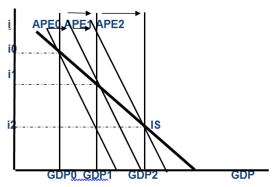
Monetary policy easing can be used to counteract the impact an independent fall in Aggregate Planned Expenditure. By making available excess funding than anyone requires at the current level of interest rates, the increase in Aggregate Supply of funding will cause interest rates to go down. We can get an idea of the implications of easing the monetary policy through the following diagram:

Tightening the monetary policy on the other hand however (as a means of fighting inflation) is temporary. The role of a tight monetary policy is very limited. It’s like

Like using weak medicine for a severe headache because unemployment isn’t handled.

Aggregate Planned Expenditure

A review of some of the preliminary formulae brings our attention to four sector surpluses, which include: the budget surplus (HY – C), which measures the amount by which the household’s current income surpasses its demand for current output. Similar concept, but now pertaining to the business sector is expressed as (BY – I).

The government surplus (GY – G) and finally (TF + F – X) which measures the foreign-trade sector’s surplus (where F is what foreign households and institutions not in the country have earned from sales of their current output and X measures what they spend on our current output). The sum of these four implicates that APE will be equal to GDP and the demand will be just right, to consume all the nation’s current output…if the sum equals 0.

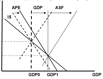
However, in order to reduce the responsiveness of the Aggregate Planned Expenditure to GDP changes (and essentially minimizing the magnitude of the potential output and employment alterations) some economic system engineered features are used. They are called Automatic Stabilizers and include: progressive net tax structures and welfare and unemployment compensation programs. Automatic stabilizers are one of the tools of the fiscal policy. The automatic stabilizers make the IS line as illustrated in the figure:

The other tool of fiscal policy is the discretionary fiscal policy which is the deliberate manipulation of government taxation, purchases and transfers in a bid to promote macroeconomic goals such as economic growth, price stability and full employment. For example, a scenario where a government changes its purchases, it may be observed that a change in Real GDP = a change in G * (1/1 – Marginal Propensity to Consume). A change in taxes, for instance a decrease in taxes will imply that: disposable income increases, consumption increases and Real GDP increases. An increase in taxes however brings about opposite outcomes.

In order to illustrate the principles of fiscal policy, we require a fiscal policy formula. Incorporating hypothetical assumptions such that ∆HT = Household tax, ∆BT = Business Tax and ∆G = change in level of government demand for current output. Further, assuming that levels of export (X) and Imports (F) (from the equation APE = C + I + G + X – F) are not directly affected by the tax and government demand changes, we get the equation ∆APE = ∆C + ∆I + ∆G. If we assume that the initial changes in Consumption, Investment and Government purchase are for the nation’s own current output and businesses allow the business savings to cater for the changes in BT, the overall fiscal-policy formula obtained is ∆APE = ∆G – 0.65∆HT – 0.35∆BT.

In the event that the government would like to raise Aggregate Planned Expenditure by a certain amount, all it would have to do is increase its purchases of current domestic output by that amount which would leave such variables as changes in household tax and changes in business tax unaltered. Other means of raising the APE would be to cut household tax or to cut business taxes (although, the business tax cut would be steeper than that of household tax.

Regardless of the means used to raise the APE by a certain amount, a common characteristic prevails: purchases of current domestic output (made by the federal government) rise relative to federal tax receipts. Whichever way you look at it, it is expansionary fiscal policy whereby the government is attempting to increase aggregate demand. And to achieve this, the government spends higher or lowers’ taxes. However, the impact of this policy will depend on many factors, for example, what else will happen to the economy? Will crowding out occur? And so on.

On the flip side however, for the federal government to reduce the Aggregate Planned Expenditure by a certain amount, it would require a combination of ∆G, ∆HT and ∆BT: for which it would require to use a restrictive policy approach. This would translate to a reduction in Federal purchases relative to tax receipts which in turn would lead to a Federal Budget Surplus and if not, reduce any current budget deficit.

At a glance, most of the variables under study majorly revolve around federal debt. The United States has had public debt since it was founded. When the federal government requires funding and borrows the treasury auctions out securities which include: bills, notes and bonds and then buy them back at their face value. In the United States, “government debts” is also referred to as the debts of the local governments. In contrast, government deficit (say annually) defines to the variation between the government’s incomes and its expenditure yearly. However, it should be noted that since the government gets most of its funding from the people, government debts are an indirect debts to the taxpayers.

Growth in the government debt is trivial compared to the anguish avoided by trying to escape the recession, but government budget deficits for ulterior reasons are fiscally irresponsible. The current federal government deficits have been severe, mostly due to the intensity of the recession.