Introduction
The main aim of this task was to establish whether there was a significant relationship between the two data sets and show whether there was a significant difference in the interventions. A descriptive statistic was done to determine the data set’s means, median, standard deviation, and variances. The pre-intervention score was 50% (0.5), and intervention for percentages, frequencies, and t-tests was conducted. The post-intervention score was 25% (0.25), indicating that the whole intervention was not statistically significant, with a p-value of.05.
Pre-Intervention
Frequencies and percentages were calculated for Q3 to Q31. The most frequently observed category of Q3 was 2 (n = 82, 50.00%), Q6 was 2 (n = 67, 40.85%), Q5 was 1 (n = 79, 48.17%), Q8 was 2 (n = 93, 56.71%), Q12 was 2 (n = 77, 46.95%) and Q4 was 2 (n = 77, 46.95%). The most frequently observed category of Q7 was 2 (n = 81, 49.39%), Q11 was 2 (n = 75, 45.73%), Q10 was 2 (n = 85, 51.83%) and Q13 was 2 (n = 78, 47.56%).
The most frequently observed category of Q14 was 2 (n = 86, 52.44%), Q18 was 2 (n = 72, 43.90%), Q15 was 2 (n = 86, 52.44%), Q17 was 2 (n = 76, 46.34%), Q16 was 2 (n = 80, 48.78%), Q19 was 2 (n = 48, 29.27%), Q20 was 2 (n = 54, 32.93%), Q21 was 2 (n = 85, 51.83%), Q22 was 2 (n = 79, 48.17%) and Q23 was 2 (n = 58, 35.37%). The most frequently observed category of Q24 was 2 (n = 83, 50.61%), Q25 was 2 (n = 81, 49.39%), Q26 was 2 (n = 82, 50.00%), Q27 was 1 (n = 84, 51.22%), Q28 was 1 (n = 96, 58.54%), Q29 was 1 (n = 79, 48.17%), Q30 was 2 (n = 83, 50.61%) and Q31 was 1 (n = 76, 46.34%).
Post-Intervention
Frequencies and percentages were calculated for Q33 to Q60. The most frequently observed category of Q33 was 1 (n = 68, 41.46%). The most frequently observed category of Q34 was 2 (n = 67, 40.85%), Q35 was 2 (n = 66, 40.24%), Q36 were 2 and 1, each with an observed frequency of 42 (25.61%), Q37 was 2 (n = 81, 49.39%) and Q38 was 2 (n = 78, 47.56%). The most frequently observed category of Q39 was 1 (n = 78, 47.56%), Q40 was 2 (n = 72, 43.90%), Q41 was 2 (n = 66, 40.24%) and Q42 was 2 (n = 74, 45.12%). The most frequently observed category of Q43 was 2 (n = 74, 45.12%), Q44 was 2 (n = 73, 44.51%), Q45 was 2 (n = 71, 43.29%), Q46 was 2 (n = 56, 34.15%), Q47 was 2 (n = 56, 34.15%) and Q48 was 4 (n = 46, 28.05%).
The most frequently observed category of Q49 was 2 (n = 41, 25.00%), Q50 was 2 (n = 72, 43.90%), Q51 was 2 (n = 70, 42.68%) and Q52 was 2 (n = 45, 27.44%). The most frequently observed category of Q53 was 1 (n = 69, 42.07%), Q54 was 2 (n = 80, 48.78%), Q55 was 2 (n = 75, 45.73%), Q56 was 1 (n = 102, 62.20%) and Q57 was 1 (n = 102, 62.20%). The most frequently observed category of Q61 was 1 (n = 98, 59.76%), Q58 was 1 (n = 101, 61.59%), Q59 was 2 (n = 67, 40.85%) and Q60 was 1 (n = 90, 54.88%).
Two-Tailed Paired Samples T-Test
A two-tailed paired samples t-test was computed to determine whether there was a significant difference between the mean differences of Total_29 and Total_59.
Assumptions
- Normality. A Shapiro-Wilk test was conducted to determine whether the differences in Total_29 and Total_59 could have been produced by a normal distribution (Razali & Wah, 2020). The results of the Shapiro-Wilk test were significant based on an alpha value of.05, W = 0.85, p <.001. This result suggests that the differences in Total_29 and Total_59 are unlikely to have been produced by a normal distribution, indicating that the normality assumption is violated.
- Homogeneity of Variance. Levene’s test was conducted to assess whether the variances of Total_29 and Total_59 were significantly different. The result of Levene’s test was significant based on an alpha value of.05, F (1, 318) = 5.10, p =.025 (Shrestha, 2020). This result suggests it is unlikely that Total_29 and Total_59 were produced by distributions with equal variances, indicating that the assumption of homogeneity of variance was violated (Conover & Iman, 2018).
Results
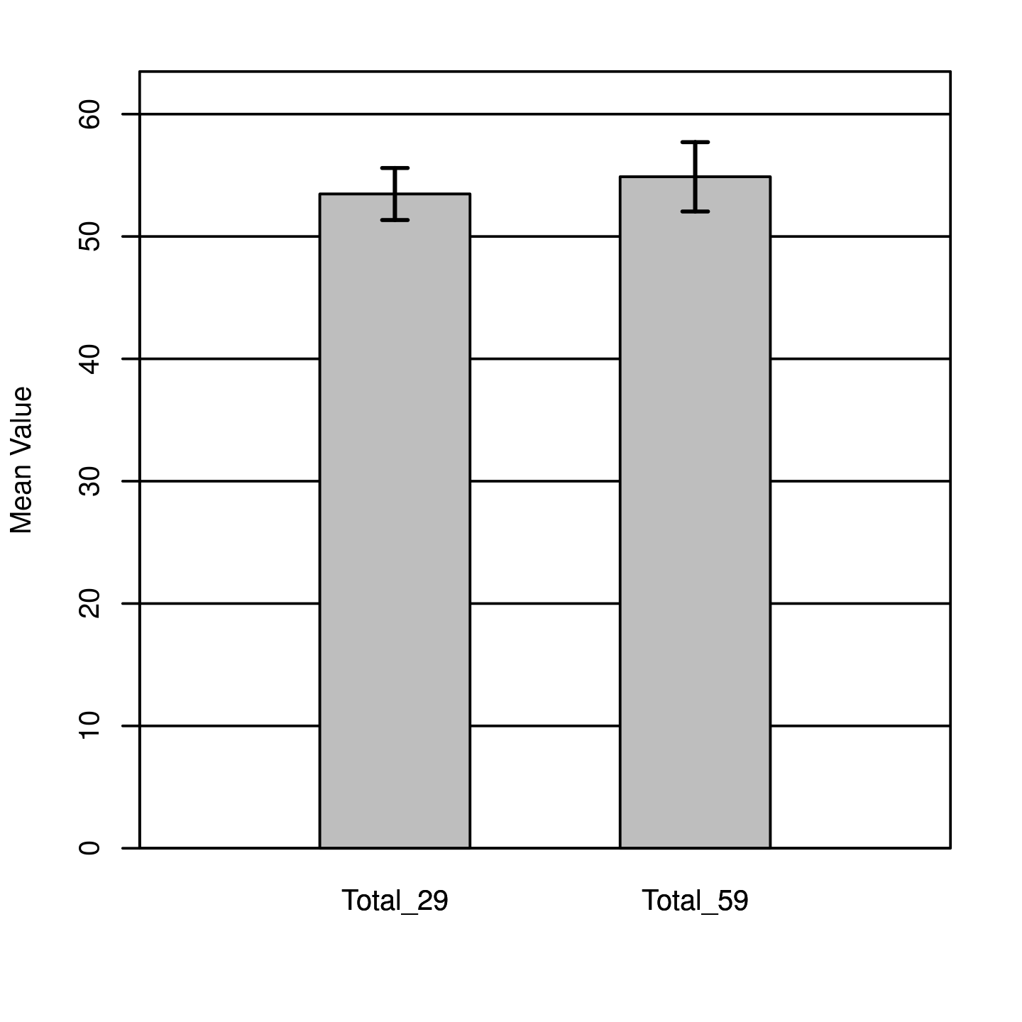
The two-tailed paired samples t-test was insignificant based on an alpha value of.05, t (159) = -1.41, p =.159, indicating that the null hypothesis cannot be rejected. This finding suggests that the difference in the mean of Total_29 and the mean of Total_59 was not significantly different from zero (Winston,2019). The results are presented in Table 1. A bar plot of the means is presented in Figure 1.
Table 1.Two-Tailed Paired Samples t-Test for the Difference Between Total_29 and Total_59

Conclusion
In conclusion, the results showed no significant difference between the two sets of observations when both descriptive and inferential statistics were conducted. In addition, the p-value of 0.05 indicated that the mean differences between Total_29 and Total_59 differed significantly from 0.
References
Conover, W. J., & Iman, R. L. (2018). Rank transformations as a bridge between parametric and nonparametric statistics. The American Statistician, 35(3), 124-129.
Razali, N. M., & Wah, Y. B. (2020). Power comparisons of Shapiro-Wilk, Kolmogorov-Smirnov, Lilliefors, and Anderson-Darling tests. Journal of Statistical Modeling and Analytics, 2(1), 21-33.
Shrestha, N. (2020). Detecting Multicollinearity in Regression Analysis. American Journal of Applied Mathematics and Statistics, 8(2), 39–42.doi: 10.12691/AJAMS-8-2-1
Winston, W. (2019). Microsoft Excel 2019: Data analysis and business modeling (6th edition). Pearson publishers.