Introduction
The present paper provides an example of statistical analysis using IBM’s Statistical Package for the Social Sciences (SPSS). The dataset under analysis was provided by the Ohio Department of Education. It includes information on ten variables from 25 school districts. This paper focuses on the analysis of two variables, which are the Percentage of Disadvantaged Students and Total Expenses per Student. The purpose of the present paper is to demonstrate how SPSS can be used to gain valuable financial information from a set of data.
Variables
The first variable under analysis is the Percentage of Disadvantaged Students in the selected districts. It is labeled “DisadvanStud(%)” and includes continuous numeric data that can vary from zero to 100. The Total Expenses per Student is labeled TotExpensePerStud is also includes continuous currency data that can meaningfully accommodate values from $0 to infinity. Both variables are ratio measurement scales with meaningful zeros, as the variables are named, ordered, with proportionate intervals between variables, and with meaningful zero values (Pyrczak, 2016). There is no missing data about these variables, which helps to avoid bias in the inferential analysis.
SPSS
SPSS is a software package used by a wide variety of researchers to analyze statistical data of various types. It was created in 1968 by SPSS Inc., which was later acquired by IBM (Foley, 2018). SPSS is valued for its straightforward command language and a thorough user manual (Foley, 2018). Even though the package is rather expensive and has free analogs, such as R Studio, SPSS is considered a gold standard for data analysis in social science, which makes if a very successful product (Foley, 2018). While the software package has a wide variety of functions, the present paper will use it only for computing descriptive statistics of two variables and visualizing the findings.
Descriptive Statistics
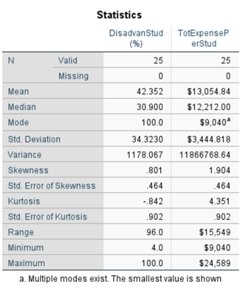
Descriptive statistics are used to summarize the information on the variables included in a dataset. This type of statistics can be used to describe an entire population or a sample from the population of interest (Kenton, 2019). Descriptive statistics can be divided into central tendency and variability measures (Kenton, 2019). The descriptive statistics of the two variables is provided in Table 1 below. The test results will be discussed in the following subsections.

Central Tendency
Central tendency measures include mean, median, and mode values. The mean value is commonly known as the average value, and it can be calculated by adding all the values and dividing them by the number of values (Pyrczak, 2016). The median is the middle value of the entire dataset when arranged in ascending or descending order (Pyrczak, 2016). The mode is the most frequent score in the dataset (Pyrczak, 2016). As seen in Table 1, the mean of the Percentage of the Disadvantaged Students is 42.35%, the median is 30.9%, and the mode is 100%. The mean of the Total Expense per Student was $13,055, the median is $12,212, and the mode is $9,040. While all of the central tendency measures have their use, they cannot be used universally. This implies that researchers need to use critical thinking to understand which of the measure represents the central tendency the best.
Variability
Variability is measured using standard deviation, variance, range, minimum and maximum variables, and kurtosis, and skewness. The range is the difference between the maximum and minimum. The minimal value of the Percentage of Disadvantaged Students is 4%, and the maximum is 100%, which makes the range large (96%). The minimal value of the Total Expense per Student is $9,040, and the maximum is $24,589, which implies that the range is also very large ($15,549). Standard deviation is a critical measure that helps to understand how dispersed the data is along the x-axis. The standard deviation of the Percentage of the Disadvantaged Students is 34.32, while the same measure for the Total Expense per Student is $3,445.
Visualization
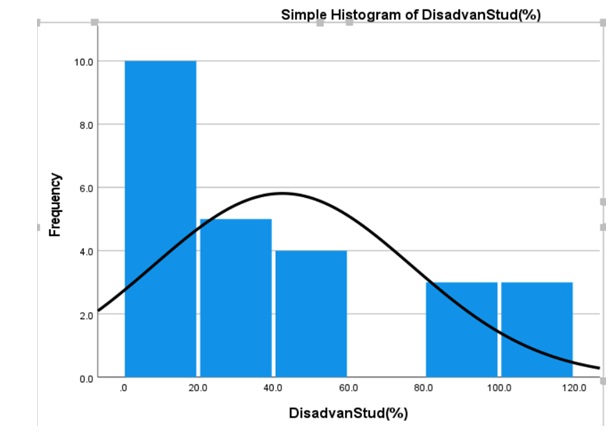
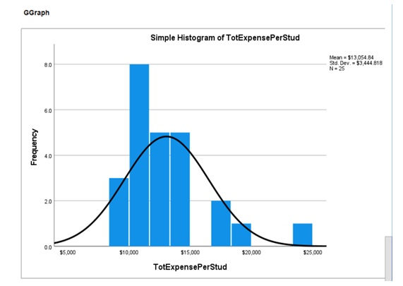
Histograms with superimposed normal curves help to visualize the distribution of data. In particular, they help to understand how different the distribution of values from the normal distribution. Figure 1 demonstrates such a histogram for the Percentage of the Disadvantaged Students. As seen from Figure 1, the distribution of values is right-skewed (skewness = 0.8) and platykurtic (skewness = -0.842). Figure 2 below pictures the distribution of values of the Total Expense per Student in a histogram. As seen in Figure 2, the curve is also right-skewed (skewness = 1.9) but leptokurtic (kurtosis = 4.35). Both of the histograms, however, demonstrate that the values do not follow the normal distribution curve.


Conclusion
Descriptive statistics helps to understand the distribution of values of variables using measures of central tendency and variability. While numeric values can help to acquire general knowledge about the sample, it is always beneficial to visualize the data using histograms or other graphical representations. SPSS is a convenient tool that helps to calculate the descriptive statistics and visualize the findings.
References
Foley, B. (2018). What is SPSS?Survey Gizmo. Web.
Kenton, W. (2019). Descriptive statistics. Investopedia. Web.
Pyrczak, F. (2016). Success at Statistics: A worktext with humor. Routledge.