Introduction
Digital image refers to a two-dimensional signal in which every digital sample is a function of two spatial coordinates x and y and whose value at that spatial point P(x,y) is the gray level of intensity at that point. Digital Images are depicted by a set of distinct sections referred to as pixels.
Just like any other raw data, digital images have no meaning before they are processed. Thus, Digital Image Processing can be said to be the process where the digital images are refined through some computer algorithms to extract information that the computer can interpret. The extracted information can thus be used to carry out further calculations or arrive at some decisions. Currently, digital image processing has found application in many different specialties; some of the important areas include medicine and surgery, space science, robotics, industrial automation, satellites, and video surveillance.
Principle Steps in Digital Image Processing
The major steps followed in digital image processing are as follows:
- Image Acquisition.
- Image Enhancement.
- Image Restoration.
- Color Image Processing.
- Wavelets.
- Compression.
- Morphological Processing.
- Segmentation.
- Representation and Description.
- Object Recognition.
In the following section, a brief description will be given about each of the above steps.
Image Acquisition
This step marks the beginning of the digital image processing exercise. In other words, image acquisition refers to the process of obtaining the image in a raw form that is readable by the computer-guided imaging device/imaging sensors. Additional hardware or some computer software that supports the reading of the raw image is used to convert the image into computer-readable format. Often the raw image data is converted into a standard image format setting the stage for further processing.
Image Enhancement
This is the second step in digital image processing. This step is one of the easiest and enjoyable in the whole digital image processing activity. Image enhancement refers to the improvement of the suppressed image detail to achieve increased visibility and mark the regions of interest in the image. Typical examples in the image enhancement process are changing the brightness and enhancing the contrast
Image Restoration
The image restoration step occurs together with image enhancement. The restoration is done by removing different types of noise that occur as a result of the imaging system or setup. The noise may be manifested as white Gaussian noise that occurs during image data transmission or may be seen as a form of blurriness or a shaking effect as a result of a bad imaging setup.
It is not possible to determine the particular amount of blurriness caused by the system and thus a probabilistic mathematical approach is needed to correct the images. The nature of the noise produced and the results required always determine the methodology to be employed.
Color Image Processing
As suggested by the name, color image processing is exclusively utilized in the processing of colored. Color image processing is a part of digital image processing in which the different concerns surrounding colored images are taken care of. This subpart of digital image processing has gained more popularity due to the widespread use of pictorial data on the internet.
Wavelets
This refers to the mathematical functions that facilitate the division of the image signal/data into tiny frequency sections. The sections are then studied by comparing them to scaled signal/image that has a similar resolution. Wavelets have different applications in digital image processing. Image compression is usually one of the most important functions of wavelets.
Compression
This is one of the important steps in image processing. Compression primarily functions to reduce the size of the image data. Compression has received a widespread application in internet pictorial representation. The internet uses a lot of pictures and compression is vital for saving the bandwidth of image data for easy transmission. Compression is also vital in the case of limited memory and storage capacity. In the past, data storage was a challenge and therefore compression always came in handy, it is however still useful in the current communication framework.
Morphological Processing
Morphological Processing functions to extract different items of interest within the image. It is often used to remove objects that are not needed in an image. Alternatively, it can be used to reconcile two sliced parts of an image. This is achieved by applying the two opposing functions of morphological processing (morphological opening and morphological closing). The two functions are based on erosion and dilation.
Segmentation
In the segmentation step, the image is divided into separate segments or regions. In other words, the respective pixels in the given regions are labeled to identify with the region. Segmentation has received widespread application especially in the area of automated computer vision applications. The extracted objects are utilized in further processing activities.
Representation and Description
Representation and description depend on other factors which may include; the desired outcome, the representation format in use, and the type of computation required. The data obtained by segmentation is often raw and only defines the regions represented by the linked pixels. Boundary representation is indicated when the external formation of the object is important in the studying of the properties inside the region. The description is often required to identify these regions before continuing with the image processing. The description is important as it points out the specific properties that are associated with the different regions of the image. Some of the common characteristics associated with the segments are texture, color, regularity, length, breadth, aspect ratio, area, and perimeter length.
Object Recognition
This is the last step of digital image processing and pertains to the classifying of the different objects regarding features and characteristics identified in the previous step. For instance, for one to differentiate between a rectangle and a square, the lengths, and breadths that cab is easily observed will be of utmost importance.
Digital Image Acquisition
Digital Image Acquisition refers to the mapping of three-dimensional (3D) world’s vision to a 2D array or matrix of image data. The acquisition of an image is achieved using an array of photosensors. There are different methods by which the photosensors can be configured or positioned to obtain the image. The light sensors liberate a voltage that is directly proportional to the light intensity that is incident on them.
An Analog to Digital Conversion (ADC) system is required to convert the liberated continuous voltage to digital form. The ADC involves two processes sampling and quantization. An image is a 2D depiction of a 3D scene as revealed by figure 2.16 (a) and every point on that 2D image is a function of two coordinate variables x and y. f(x,y) represents the light intensity at that given point. Thus for an image to be digitized, the x-y coordinates and the intensity and the intensity value of the amplitude also need to be digitized. The digitizing of the x-y coordinates is referred to as sampling while the digitization of the amplitude is referred to as quantization.
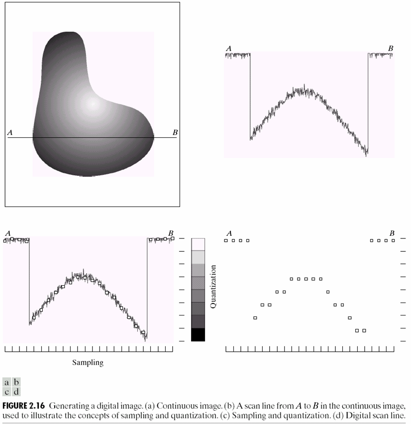
Figure 2.16(b), the continuous voltage signal which is directly proportional to the light intensity can be seen. This is also revealed along with the line segment AB as shown in figure 2.16(a). Digitization of the signal should be performed along both dimensions now. Samples of the signal are taken at regular intervals along the horizontal direction and hence digitization along the x-direction is acquired. This form of digitization is referred to as sampling. The sample points at regular intervals are represented as white boxes along with the intensity signal. These points or boxes that are aligned vertically should then be digitized.
As shown in figure 2.16(c), the vertical scale can be separated into eight different grayscale levels. During the digitization process, the vertical points are assigned appropriate grayscale values depending on the position in which they fall. The process of quantization which refers to assigning discrete or quantized values to vertical sample points is shown in figure 2.16(d). Three methods can be used to assign the discrete values to the vertical samples. The methods are approximation, floor and ceiling schemes. In addition, several ways can be used to sample the data and this often depends on the arrangement of the light sensors.
Thus far, the basic processes involved in digital image acquisition have been explained. This section will now examine what is observed if the total numbers of samples for a given image are increased or decreased. The effect of increasing and decreasing gray levels will be captured briefly in the discussion. It is imperative to note that the term sample is substituted by the term pixels when discussing images. The following figures are important for a better understanding of the effect brought about by sampling and change in the number of samples.
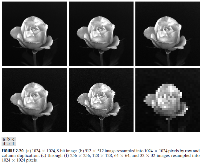
Figure 2.20 (a) is a picture of a flower taken at 1024×1024 pixels. This implies that 1024 pixels for both the x and y-axis have been used to represent the image. The same image is seen in figure 2.20(b) but with the pixels reduced to 512x 512 and then upsampled again to 1024×1024 pixels resolution. The same can be seen in the other figures, 2.20 (c) to (f) in which the initial images were taken at 256, 128, 64, and 32 respectively, and then their resolutions increased to 1024×1024. In the sampling, the nearest neighbor method was utilized.
Up-sampling entails approximation and therefore if any information is lost during the process it cannot be restored to its original form. This is evident in the following images but it is more pronounced in the last two cases in which a disturbance is seen in both the structure and shape o the flower. Therefore the aggregate number of samples used to represent an image has a big influence on the information and details in the image.
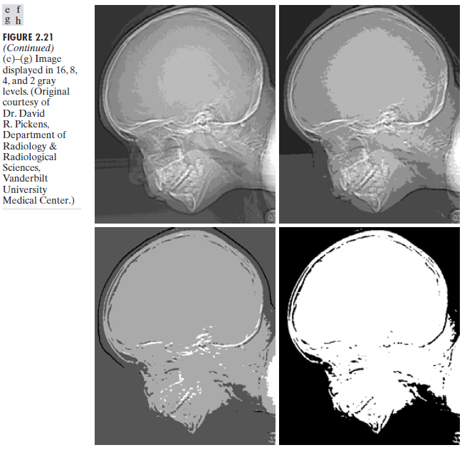
In this section, the effect of quantization levels on an image will be seen. For a clearer understanding, figure 2.21 will be used. The first figure, (a), shows an X-ray image of human skull taken at 452×374 pixels and is represented by 256 different grayscale levels. In other images, 2.21(b) to (f) the same pixels resolutions have been used in taking the pictures but the gray scale levels are 128,64,32,16,8,4, and 2 respectively This implies that a higher number of pixels enables one to have a greater choice of gray shades for a given sample or pixel representation.
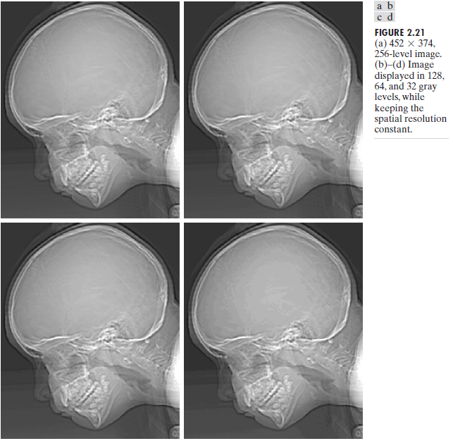
Note that the same resolution has been used for all the images and therefore the structuring and the shape of the skull is intact throughout to the 2gray level image. However, due to the limited gray levels as from 2.21(a) to 2.21 (f) the actual color information of every object or location in the image has diminished. This is a typical example of how the availability of gray scale levels in the particular imaging system affects the representation of the image and its contents.
Alpha Blending
Alpha blending is done by the MATLAB code. The code is given in the form of an equation and is used in the analysis of a picture.
The equation reveals that many lines have been commented out. These lines are utilized in the alpha blending for different alpha values that range from 0.1 to 0.9 with an increment of 0.1 and hence nine different images as Y1, Y2…Y9. This part of the code displays the resultant images as a single function. To do this, the show and subplot functions are used. The typical l output is depicted in the figure below. The actual code which generates an output of a fixed code of alpha is composed of only the first six lines. The remaining lines are used for analyzing the behavior of the blending.
At this point, we will try to analyze the effect associated with changing the values of the alpha code shown above. As shown by the equation, image Y results from the scaled addition of image A and image B. If the Above equation is divided into two factors that are being added then the result will be;
F1 = αA and F2 = (1-α) B => Y = F1 + F2;
The net effect of Factor F1 will decrease for lower values of alpha while factor F2 will increase for lower values of alpha and the reverse is true. Thus when the two factors are added the value of alpha will determine which factor to dominate. This can be seen from the image above; the lower the value of alpha the greater the effect of F2 and hence the image in variable B dominates. Higher values of Alpha lead to the suppression of F2 and thus F1 is observed.
%% Alpha Blending
A = double(imread(‘subject01.normal’));% Reading first image.
B = double(imread(‘subject02.normal’));% Reading second image.
alpha = 0.5;%alpha can have any value btw 0 and 1 change value & observe
Y = uint8(alpha.*A + (1-alpha).*B);%Applying alpha blending equation.
figure;% Creating Graphics Object.
imshow(Y);%Displaying the result of alpha blending
%% If one wish to see results for different values of alpha (optional)
% Y1 = uint8(0.1.*A + (1-0.1).*B);% Calculating result for alpha = 0.1
% Y2 = uint8(0.2.*A + (1-0.2).*B);% Calculating result for alpha = 0.2
% Y3 = uint8(0.3.*A + (1-0.3).*B);% Calculating result for alpha = 0.3
% Y4 = uint8(0.4.*A + (1-0.4).*B);% Calculating result for alpha = 0.4
% Y5 = uint8(0.5.*A + (1-0.5).*B);% Calculating result for alpha = 0.5
% Y6 = uint8(0.6.*A + (1-0.6).*B);% Calculating result for alpha = 0.6
% Y7 = uint8(0.7.*A + (1-0.7).*B);% Calculating result for alpha = 0.7
% Y8 = uint8(0.8.*A + (1-0.8).*B);% Calculating result for alpha = 0.8
% Y9 = uint8(0.9.*A + (1-0.9).*B);% Calculating result for alpha = 0.9
% figure; % Creating Graphic Object
%%% Displaying all resultant images in one figure using subplot and imshow
% subplot 331; imshow(Y1); title(‘alpha = 0.1’);
% subplot 332; imshow(Y2); title(‘alpha = 0.2’);
% subplot 333; imshow(Y3); title(‘alpha = 0.3’);
% subplot 334; imshow(Y4); title(‘alpha = 0.4’);
% subplot 335; imshow(Y5); title(‘alpha = 0.5’);
% subplot 336; imshow(Y6); title(‘alpha = 0.6’);
% subplot 337; imshow(Y7); title(‘alpha = 0.7’);
% subplot 338; imshow(Y8); title(‘alpha = 0.8’);
% subplot 339; imshow(Y9); title(‘alpha = 0.9’);
Histogram Equalization
This is one of the methods used in digital image processing to enhance the contrast of an image. “Histogram of an image is a vector equal to the length of a total number of grayscale levels in the image.” When using a grayscale level of let’s say 256 and the histogram has an indexing range of between 0 and 255, then the histogram vector will be;
H(i)=Total Number of Pixels in the image with grayscale value “i”;
Therefore when a histogram of low contrast images is plotted and observed it is visualized that the histogram has high peaks within a small range of grayscale “The histogram usually has a high density of greater values over a certain range instead of a spreading behavior over the whole grayscale range.”. The basic objective is usually to ensure that the histogram values are distributed over the whole grayscale. This is achieved by “linearization of commutative distribution function (CDF)” of the image x. If P is a pixel with a grayscale value P (i) then CDF at i is determined by.
A function such as y= T(x) is required to obtain an image y with equalized histogram. “Where T is some transform function such that the CDF of y is more or less linear and could be defined as follows.”.
Where K represents a constant that has a value that will make it possible to determine a relationship that satisfies the following
The general formula for the transformation is given below.
In the equation, M and N represent the number of rows and columns in the image respectively. L is the total number of available grayscale levels.
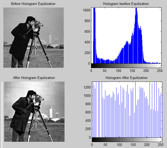
The written MATLAB is utilized while increasing the contrast of the “cameraman”. MATLAB image processing toolbox comes with a function referred to as “his tea” that is utilized in equalizing the histogram thus increasing its contrast. The image depicting a cameraman has been processed using MATLAB that includes the function and the results can be observed. A corrected version of the image can be seen. The histograms of both images are shown below the images.
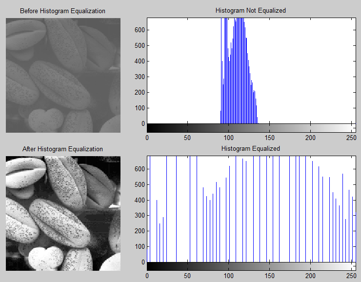
For the histogram depicting the cameraman, it is seen that most of the pixel values fall between 100 and 180. The grayscale values have a small range of approximately 0 to 15 where the peaks for the histogram plot are located. On observing the image after the histogram of the cameraman, it is seen that the image has better contrast and a similar effect is seen by the spreading of the histogram. The second example shows a better effect of enhancing the contrast.
The image after the histogram equalization shows a better contrast than the original image. From the histogram, it is seen that all the pixels fall between 90 and 135 grayscale values. This explains why the original image appears a bit dull; all the pixel values are close together and it is difficult to differentiate the regions of the image. By spreading the pixel values over the whole grayscale a more or less equalized histogram is achieved leading to better contrast.
%% Histogram Equalization method if contrast enhancement
I = imread(‘cameraman.tif’); % Reading the image
%%% One can change the input image and observe the result.
J = histeq(I);% Applying Histogram Equalization
%%% Displaying actual image and contrast enhanced image using his
togram
%%% equalization and their respective histograms as one figure.
subplot 221
imshow(I); title (‘Before Histogram Equalization’);
subplot 222
imhist(I); title (‘Histogram Not Equalized’);
subplot 223
imshow(J); title (‘After Histogram Equalization’);
subplot 224
imhist(J); title (‘Histogram Equalized’);
References
Gonzalez RC, Woods RE. Digital Image Processing, 2nd Ed. Prentice-Hall, 2002.
An introduction to Wavelets [document from the internet] 2010. Web.
T. Acharya and Ajoy K. Ray, Image Processing Principals and Applications Hoboken , NJ : Wiley-Interscience, 2005.
Histogram equalization [document on the internet] Wikipedia; 2010. Web.
Fisher R, Dawson HK, Fitzgibbon A, Trucco C. Dictionary of Computer Vision and Image Processing. New York: John Wiley.
Milan S, Vaclav H and Roger B. Image Processing, Analysis, and Machine Vision. New York: PWS Publishing; 1999.