The decrease in consumption of electricity and heat produced by conventional methods should decrease the transition to cleaner sources, but in practice, the reality is far from that. Under profound climatic changes and cold weather conditions, the critical issue of survival and maintenance of the regular quality of life is the heating of houses, depending on how warm or cold the house will be. When the outside temperature decreases rapidly due to seasonal changes, heating is practically the only and one of the most common heating energy for households. The quality of such heating is determined by a combination of factors, including the deterioration of the house, thermal insulation, the number of people living in the household, exposure to wind, and others. This case study examines the case of Dupree Fuels Company, which sells heating oil to residential homes. The company’s main task is to develop a forecasting model that determines when customers run out of products and to offer its services promptly. In the current work, statistical analysis based on linear regression was conducted to investigate such forecasting possibilities.
Regression analysis initially requires an examination of the nature of the variables used. Oil consumption, measured on a continuous numerical scale, is the dependent factor. The number of degree days (DD), which determines the absolute difference in the year when the temperature was below the required minimum, should be used as the independent variable. The number of people living in a household can also be used for regression analysis, as this can demonstrate the effect of family size on oil consumption. The home index measured not on a ratio but on an interval continuous scale can also be used as an independent variable under the regression analysis assumptions (SL, 2021). Thus, it makes sense to perform individual and multiple regression analyses to identify the aggregate effect of independent factors. To perform such an analysis, IBM SPSS is used to automatically determine the significance of the constructed model and the values for the equation coefficients.
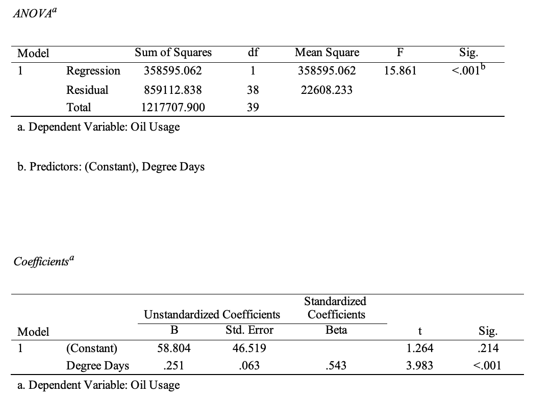
The first step of the regression analysis is to evaluate the effect of DD on household consumption of heating oil. Table 1 shows the regression results for a sample of 40 households. As follows from the ANOVA part of this table, the linear regression model is significant as long as the corresponding p-value is below the critical alpha level (.05). In other words, since the calculated p-value (<.001) is significantly lower than.05, the null hypothesis must be rejected, and thus the resulting model is significant, that is, the DD variable has a statistically significant effect on household heating oil consumption.
The coefficient of determination, which demonstrates the reliability of the constructed model, was.294, which means that only 29.4 percent of the variance in the data could be explained by the model, which is not a high figure. In the Coefficients section, one should pay attention to exactly what effect DD has on heating oil consumption. Attention should be paid to the significance of the coefficient: for the DD variable, the p-value was calculated to be <.001, which is below the critical alpha level (.05), which means that the null hypothesis of no effect of this variable on Oil Usage should be rejected. For the intercept ratio, the p-value was.214, which is higher than.05, so the intercept was not significant. Thus, the overall significance of the model and the DD coefficient (see Table 1) were confirmed. The relevant value of the DD in the linear equation, namely the slope of the straight line, is equal to 0.251, which indicates that an increase in DD for every unit leads to an increase in heating oil consumption by 0.251 points, that is, an upward linear trend characterizes the relationship between the two variables. The model can be used for prediction because with any value of DD, it becomes possible to determine Oil Usage according to the equation Oil Usage = 58.804 + 0.251∙DD.

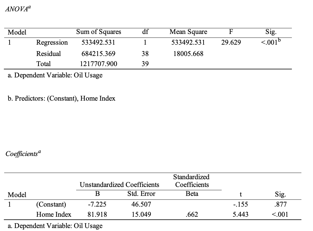
The second factor to check is the Home Index as a measure of its aggregate quality characteristics. The higher this index is on a five-point scale, the more resources a household may need due to internal and external structural, demographic and environmental factors. Table 2 reports the results of the regression performed. One can see that the p-value (<.001) for the model as a whole is below 0.05, so the model can be considered significant. The coefficient of determination in this case was higher and was 0.438, which means that up to 43.8% of the variance could be explained by the model. At the same time, for the Home Index coefficient, the p-value was lower than 0.05 and higher for the intercept. This means that the Home Index coefficient was significant, unlike the intercept. Thus, the results of the analysis show that a one-unit change in the Home Index on a five-point scale results in an 81.918-point increase in consumption. This model can be used for forecasting because, for any value of the Home Index, Oil Usage will be determined according to the equation Oil Usage = -7.225 + 81.918∙HI.

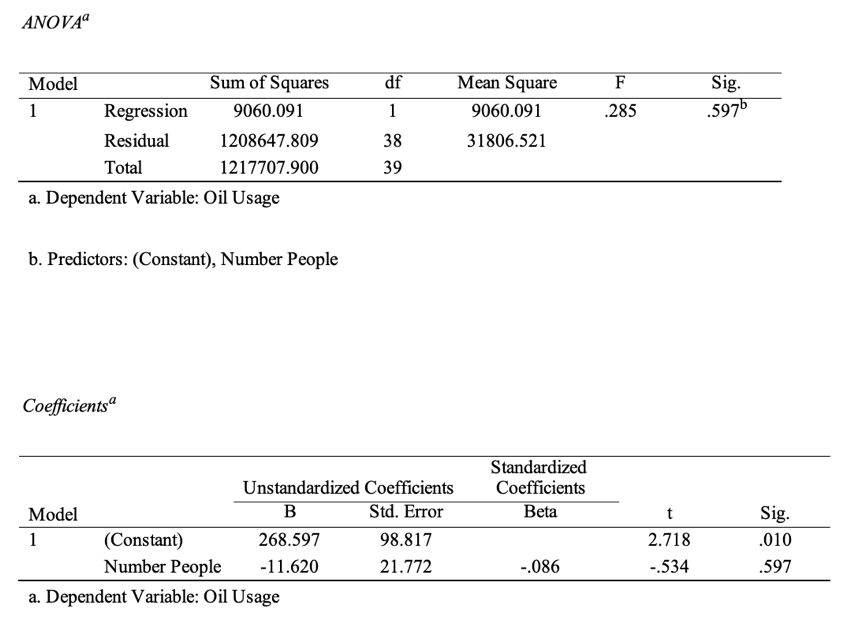
Finally, among the isolated variables of interest was measuring the effect of the number of people living in the house on food consumption. Reference Table 3 shows that neither the equation coefficient in isolation nor the regression model itself were statistically significant because the corresponding p-values were 0.597, that is, above.05. This implied that the effect of one variable on another was not confirmed, and the calculated numbers may have indicated an overlap or error (Kim, 2019). The unreliability of the model is also confirmed by the low coefficient of determination, equal to 0.007, or 0.7% of the explained variance. Thus, the number of people living in the house was not a significant predictor of oil consumption, so this model should not be used to predict.

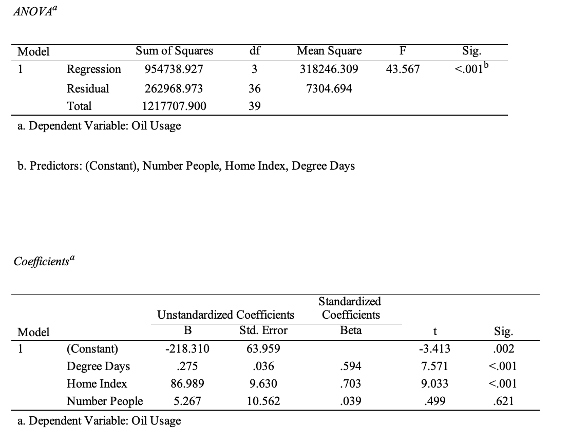
Multiple regression made sense because it could lead to different results if the independent variables interacted with each other. Table 4 shows the results of the multiple regression with the three predictors as independent factors. One can see that the model itself was statistically significant because the p-value was below.05, with each factor except the number of people also showing significance. This model yielded the highest coefficient of determination, explaining up to 78.4 percent of the variance. For DD and Home Index, the corresponding p-values were <.001, that is, below.05. As expected, based on the individual linear regression results, the model itself, DD, and the Home Index variables were significant, while the number of people living in the household remained an insignificant factor. In other words, removing this variable would not have had a significant effect on the regression results. The upward trend in the regression persisted, with a marked increase in the strength of this effect for both significant variables. This suggests that the combination of DD and the house index has a synergistic effect on oil consumption compared to each factor separately. This model can be used to predict changes in oil consumption using the equation Oil Usage = -218.310 + 86.989∙HI + 0.275∙DD.

In conclusion, using statistical analysis to evaluate the relationship between variables is a dependable, data-driven approach to decision-making. In the current paper it should evaluate which factors significantly affect household oil consumption. It was found that the number of degree days and household index significantly determine oil consumption, while the number of people living in the house does not. This result can be used to develop Dupree Fuels Company’s commercial solutions further to ensure continued sales to customers.
Reference List
Kim, J.H. (2019) ‘Multicollinearity and misleading statistical results.’, Korean Journal of Anesthesiology, 72(6), pp. 558-569.
SL (2021) Linear regression analysis using SPSS Statistics. Web.