Introduction
Fourier Transform is an important process in digital image processing. It applies to various aspects in the field of digital image processing and can be used for both “one dimensional (ID) signals such as sound and two-dimensional signals (2D) such as images”. The digital transform analysis brings to light several concealed aspects of signals which are usually not seen. For the case of 1D, the concealed features may not be seen in the time domain or spatial domain for both 1D and 2D.
Through the Fourier analysis, the magnitude of every frequency element is determined and thus it reveals the main contributing frequencies. In addition, it indicates the phase at which the various frequency components are. The Fourier analysis has received a major application in the process of image filtering and processing in which it facilitates the identification of the main contributing frequencies in a signal (image).
This in turn facilitates the differential analysis of a signal (image), enabling the removal of unsuitable frequencies to modify the appearance of the image. Digital image filtering is synonymous with the Fourier analysis which is the main process utilized in this area of digital image processing. This study seeks to analyze the transformation of an image to the Fourier domain using the “Fast Fourier Transform (FFT) algorithm”. FFT algorithm is a fast algorithm that is utilized in the calculation of Discrete Fourier Transform (DFT). In this paper, the steps followed in designing some basic filters will be discussed. The filters such as the “ideal low pass, high pass filters, and the Gaussian low filters” will then be applied in filtering the image used in the study.
Discrete Fast Fourier Transform in MATLAB
Comment on each statement above
This prompts the deleting or erasing of all the displayed data in the MATLAB workspace.
This prompts the closure of all toolboxes or other related windows while keeping the MATLAB window open.
This implies the reading of an image whose name may be img.jpg. The ‘f’ refers to the 2D matrix variable in which the image will be stored.
The above code refers to the use of two functions whereby the output is by the first function and the input by the second. The conversion of the image matrix in variable ‘f’ to the double class is represented by the function ‘fft2’. This function uses the fast Fourier transform algorithm to calculate the Fourier transform. The results are then stored in the variable ‘f’.
This indicates that the absolute of each element in the matrix F will be established and the findings stored in the variable ‘S’. It is important to note that the function “abs” calculates the complete value of every element in the matrix F. This is essential because after ‘f’ has undergone Fourier Transform the resultant matrix often has complex numbers that cannot be shown. Therefore the absolute value is found and displayed as a square root in the case of complex numbers.
This function is used to shift the frequencies from the periphery or the corners to the center of the frequency spectrum.
This function is used to make the frequencies in the spectrum more visible. This is done by applying the log of the values in the Fourier spectrum which enables them to fall in the range of between 0 and 255.
The first statement implies that if the results are shown as subplots in the upper left corner then the original image in ‘f’ is displayed. The second implies that if the results are shown in the right upper corner then the Fourier Spectrum with the absolute Frequencies is displayed. The third refers to the showing of results in the left lower corner to the center of the spectrum; in this case, the image will be displayed. Finally, on the lower right corner, the log-transformed frequency spectrum with more visible frequencies will be displayed.
What “fftshift” is used for? What will happen if ignore this step?
When a Fourier Transform is performed on a 1D signal, the DC element is placed at the first index of the Transform, followed by the next frequency bin in the spectrum and this proceeds that way. The same is observed when Fourier Transform is performed on 2D signals (Images). For this to occur, the DC component is usually placed at the upper left corner of the initial index of the 2D matrix of Fourier Transform. Other frequency components which range from low to high are positioned relative to the DC component respectively. The results of a “Fourier Transform are displayed as asymmetrical frequency spectrum,” the other components, the DC component included, are positioned at the four corners of the frequency rectangle/spectrum.
The generated results are often 100% correct, however, the frequencies should be shifted from the corners to the center of the Frequency spectrum to achieve increased visibility and thus have a better analysis. The “fftshift” function in the image processing toolbox is used to carry out this process. Before this is done the frequencies usually appear increasingly from the corners to the center of the spectrum. The function “shift” simply reverses this and thus the frequencies increase from the center to the corner.
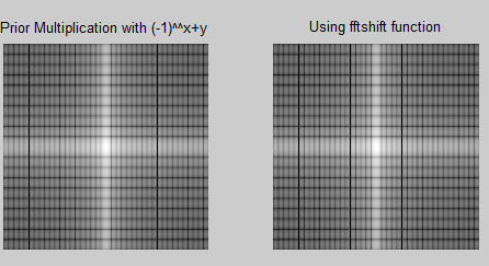
The function of “fftshift” can be replaced by multiplying the input image by (-1)^(x+y) before computing FFT. Rewrite the program by this means and report if you get the same results.
The program below shows how multiplying input image by (-1)^(x+y) will lead to the same results obtained by the function “shift”. The code and the output are shown in the figure.
%% Multiplying by (-1)^x+y and acquiring the same result as fftshift
f=double(f); % Converting the image data in f to double data type
[m,n]=size(f);% Finding size of the image f
T = zeros(size(f));%% Creating an empty matrix of size of f
for i =1:m
for j=1:n
T(i,j)=f(i,j).*((-1).^(i+j));% Multiplying f(x,y) by (-1)^(x+y) and storing in T
end
end
Ft = fft2(T);% Taking FFT of the image in T (New matrix obtained from above multiplication)
Fct = log(1+abs(Ft));%% Taking Log transform
figure;
% Displaying the Fourier Spectrum as image.
subplot 121;imshow(Fct,[]); title(‘Prior Multiplication with (-1)^^x+y’);
% Displying the image when fftshift was used
subplot 122;imshow(S2,[]); title (‘Using fftshift function’);
Write a program to implement the following steps
Use the above image to implement the following steps:
- multiplying the image by (-1)^(x+y);
- computing the DFT using “fft2”;
- take the complex conjugate of the transform;
- computing the inverse DFT;
- multiplying the real part of the result by (-1)^(x+y);
- Write the resulting matrix to an image file.
- Compare the result image by using “subplot” function
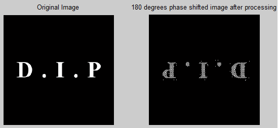
The code for the above task is given below followed by the result acquired.
clc
clear all;
close all;
X=imread(‘.img02.jpg’,’jpg’);% Reading the image
figure; imshow(X);axis equal;axis off;
[m,n]=size(X);%% Finding the size of the image
Y = size(X);%% Creating a matrix same in size as that of X
Z = size(X);%% Creating a matrix same in size as that of X
for i = 1:m
for j = 1:n
Y(i,j)=X(i,j).*(-1)^(i+j);%% Multiplying X(x,y) by (-1)^(x+y) and storing in Y
end
end
F= fft2(Y);%% Taking FFT
Fc = conj(F);%% Taking Complex Conjugate
Ix = ifft2(Fc);%% Taking Inverse Fourier Transform
Ir = real(Ix);%% Taking out the real part from the inverse Fourier Transform
for i = 1:m
for j = 1:n
Z(i,j)=Ir(i,j).*(-1)^(i+j);%% Multiplying Ir(x,y) by (-1)^(x+y) and storing in Z
end
end
imwrite(Z,’result_Q2.jpg’);%% Writing the resultant image.
figure;%% Creating an image object
% Displaying original image as subplot
subplot 121; imshow(X); title(‘Original Image’)
% Displaying the result after processing as other subplot
subplot 122; imshow(Z); title(‘180 degrees phase shifted image after processing’)
Surface Plotting
Comment each statement above and what is the difference between “mesh” and “surface”?
clc
Clear Screen
clear all;
This will delete all variables of all data types and classes in the MATLAB workspace.
close all;
This will close all figures toolboxes or any other window while the main MATLAB window will be kept open.
[X,Y] = meshgrid(-2:.2:2, -2:.2:2);
This will generate X and Y arrays for 3D plot
Z = X.* exp(-X.^2 – Y.^2);
The values to be assigned to as the magnitude along the third dimension are being calculated for different values of X and Y
figure;
Creating Graphics Object
surf(X,Y,Z);
Creating Surface Plot for the values of X, Y and Z
figure;
Creating Graphics Object
mesh(X,Y,Z);
Creating Mesh Plot for the values of X, Y and Z
Surf and Mesh Plots
Surf and mesh plots are utilized in the analysis and the visualization of 2D data in three dimensions (3D). The two functions create a 3D parametric surface for data that is included as 2D. The basic form of these functions is shown below.
Function (Z);
This function can be in both surf and mesh plots. In this function, the magnitude of the value of the elements in the matrix Z at the respective x-y coordinates is represented by the height of the plot along the Z dimensions. In this case, the respective value marks on the X and Y axis are set by default settings of MATLAB. However, a plot in the desired range of X and Y axis lengths with scaling marks can be obtained by specifying the values of X and Y matrices.
The function also allows the controlling of the colormap property to display the 3D plot. “The height of the data in Z matrix is directly proportional to the colormap chosen and is represented by that color in the 3D plot.” The greatest value in the Z matrix is automatically mapped onto the first color in the colormap while the lowest value is mapped to the last color and the while values are linearly mapped. The two functions also support the representation of the contours under the 3D plots. A contour which “refers to a boundary around the regions sharing the same pixel intensities is drawn using the contour command in MATLAB.”
Both surf and mesh plots serve the same purpose and can be used interchangeably on some kind of input. The main difference between the mesh and surf plot lies in the area that is filled with color. For the mesh plot, the wireframe is filled with color in what is referred to as faceted shading. Thus the mesh plot forms the wireframe representation of the parametric values of Z in which the area between the wireframe is empty. While in the surf plot the regions between the wireframe are filled with color and not the wireframe. Thus a surf plot depicts a parametric representation of the data values in Z.
Low Pass Filter in Frequency Domain
Write a program to implement an ideal low pass filter
In instances when the D0 is a particular nonnegative number and D(u,v) is the distance from the point (u, v) to the center of the filter.
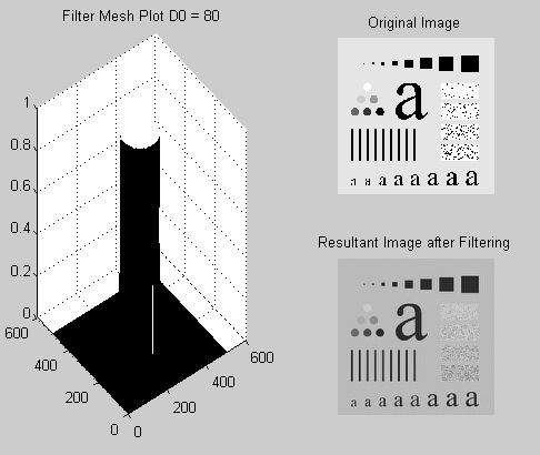
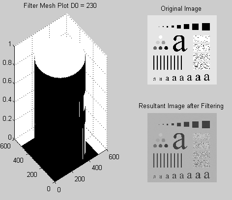
Plot the filter using “mesh” or “surface”; filter the test image “img03.jpg” with an ideal low pass filter with cutoff frequencies set at radii values 5, 30, 80, and 230.
Below is the code that represents the ideal low pass filter. The code can be modified to reflect changes in values of the radial distance DO.
%% Q# 4 Ideal Low Pass Filter
clc
clear all;
close all;
I = imread(‘img03.jpg’);%% Reading Input Image
[m,n]=size(I);
D0 = 80;%% CHANGE the distance parameter and observe the result
[u,v]=dftuv(m,n);%% Creating
d= sqrt(u.^2 + v.^2);%% Calculating the distance
Lfilt = double(d <= D0);%% Creating filter as defined
Lfilt_s = fftshift(Lfilt);
Iff = fft2(I);%% Fourier Transform of the image
Rf = Iff.*Lfilt; %Multiplying filter with the image both in Fourier Domain
R = ifft2(Rf); % Inverse fourier transfrom of the above filtered image
figure
% Displaying the final result
subplot (2,2,2); imshow(I);title(‘Original Image’)
subplot (2,2,4); imshow(R);title(‘Resultant Image after Filtering’)
subplot (2,2,[1,3]); mesh(Lfilt_s);title(‘Filter Mesh Plot D0 = 5’)
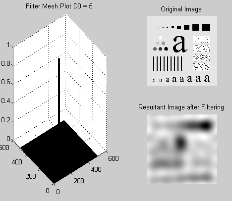
The outputs at different values of distance D0 are given as follows
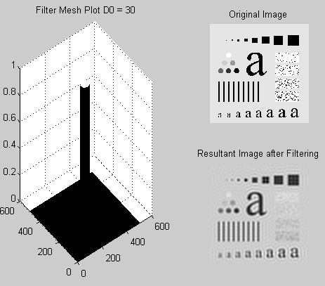
Write a program to implement the Gaussian low pass filter

Plot the filter using “mesh” or “surface”; filter the test image “img03.jpg” with ideal low pass filter with cutoff frequencies set at radii values 5, 30, 80 and 230.
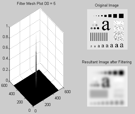
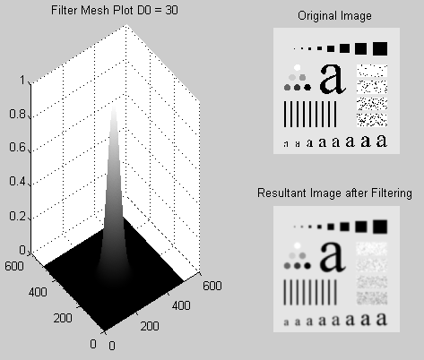
The Gaussian Low pass filter code is given below. The values of the radial distance can be modified easily using the code.
%% Q# 4 Gaussian Low Pass Filter
clc
clear all;
close all;
I = imread(‘img03.jpg’); %% Reading Input Image
[m,n]=size(I);%% finding size of image and stroing in m and n
D0 = 5;%% CHANGE the distance parameter and observe the result
[u,v]=dftuv(m,n);%% Creating
d= sqrt(u.^2 + v.^2);%% Calculating the distance
G_Lfilt = exp(-(d.^2)./(2*(D0^2)));
G_Lfilt_s = fftshift(G_Lfilt);
Iff = fft2(I);%% Fourier Transform of the image
Rf = Iff.*G_Lfilt; %Multiplying filter with the image both are in Fourier Domain
R = ifft2(Rf); % Inverse fourier transfrom of the above filtered image
figure;
% Displaying the original image
subplot (2,2,2); imshow(I);title(‘Original Image’)
% Displaying the final result
subplot (2,2,4); imshow(R,[]);title(‘Resultant Image after Filtering’)
% Displaying the mesh plot of filter tranfer function
subplot (2,2,[1,3]); mesh(G_Lfilt_s);title(‘Filter Mesh Plot D0 = 5’)
The output as the filtered image for different values of radial distance D0 is shown in the following figures.
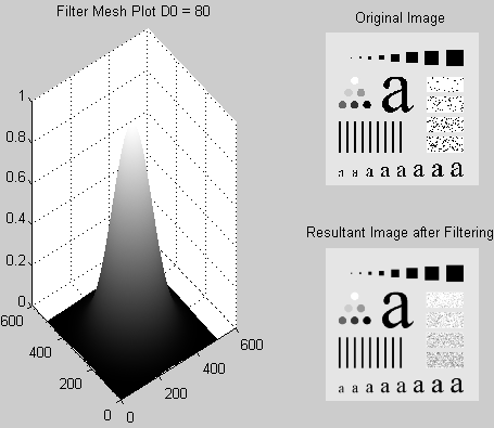
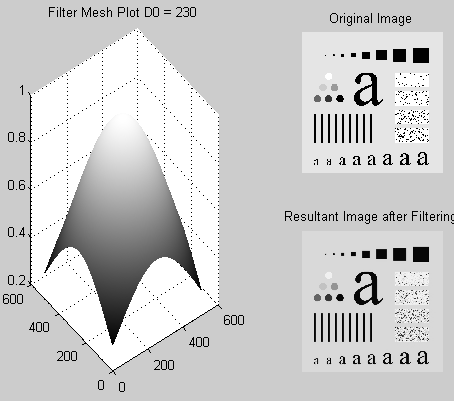
The “dftuv” function has been used to design the above filters [3]. The “dftuv” function is used to compute the meshgrid frequency matrices U and V which have the same size as that of the filter matrix.
The code for the “dftuv”function is shown below.
function [U, V] = dftuv(M, N)
% Set up range of variables.
u = 0:(M – 1);
v = 0:(N – 1);
% Compute the indices for use in meshgrid.
idx = find(u > M/2);
u(idx) = u(idx) – M;
idy = find(v > N/2);
v(idy) = v(idy) – N;
% Compute the meshgrid arrays.
[V, U] = meshgrid(v, u);
High Pass Filter in Frequency Domain
The high pass filter can be obtained from low pass filter in frequency domain by,

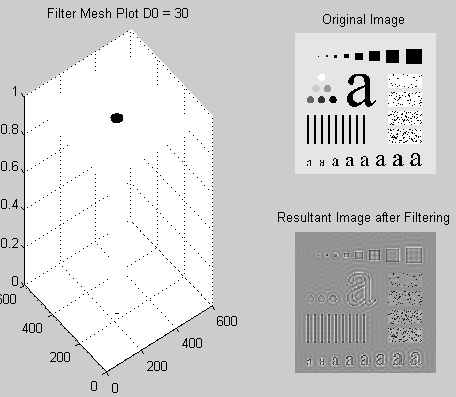
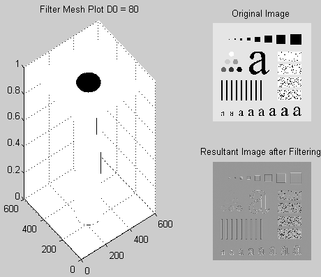
Apply the high pass filter to the “img03.jpg” and report what you get.
The code for Ideal High pass filter is given below where the values for D0 can be easily modified.
%% Ideal High Pass Filter
clc
clear all;
close all;
I = imread(‘img03.jpg’); %% Reading Input Image
[m,n]=size(I); %% finding size of image and stroing in m and n
D0 = 5;%% CHANGE the distance parameter and observe the result
[u,v]=dftuv(m,n);%%
d= sqrt(u.^2 + v.^2);%% Calculating the distance
Lfilt = double(d <= D0);%% Creating filter as defined
Hfilt = 1-Lfilt;%% Generating High pass filter from low pass filter
Hfilt_s = fftshift(Hfilt);%% Shitfing the DC componnet to centre
Iff = fft2(I);%% Fourier Transform of the image
Rf = Iff.*Hfilt; %Multiplying filter with the image both are in Fourier Domain
R = ifft2(Rf); % Inverse fourier transfrom of the above filtered image
figure
% Displaying the original image
subplot (2,2,2); imshow(I);title(‘Original Image’)
% Displaying the final result
subplot (2,2,4); imshow(R,[]);title(‘Resultant Image after Filtering’)
% Displaying the mesh plot of filter tranfer function
subplot (2,2,[1,3]); mesh(Hfilt_s);title(‘Filter Mesh Plot D0 = 5’)
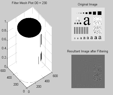
For different values of D0 we have the results as shown in the following figures.
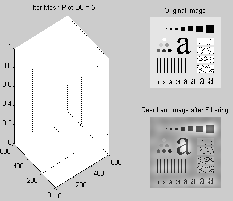
Discussion and conclusion
In this study, the behavior of the image in the frequency domain also known as the Fourier Transform has been shown. Fourier Transform facilitates the analysis and observation of different frequency components and thus revealing their respective effects or contributions to an image. The study has also revealed how various operations are carried out in the Fourier Domain. The different effects imparted on an image after processing have also been shown.
It has been shown that using the surf and mesh plots a 2D data matrix can easily be displayed in a 3D plot. Thus a better observation and understanding is achieved by observing the 2D data in a 3D perspective. This function is particularly vital in observing the Fourier spectrum of an image and analyzing the behavior of the different designs of filters. For instance, the magnitude of the responses of the cut-off frequencies and other similar properties can be analyzed clearly in a 3D display. In this study three filters were designed; two ideal low pass filters and a Gaussian low pass filter. It has been shown that when a low pass filter is applied to an image it produces a blurring effect.
This is seen in all the low pass filters (Gaussian, Ideal, Butterworth, and others). However, the different types of filters have other specific effects which may be advantageous or disadvantageous and thus they vary in usage. The smaller the radii of the low pass filters greater the blurring effect. The high pass filters produce an effect that is opposite to this. For instance, when an image is passed through the high pass filter the resultant image will have objects with sharper edges, this is because high pass filters allow high-frequency elements to pass. The larger the radius of a filter the sharper the image, however, this may lead to loss of color information because the color is contributed by low-frequency components (slowly changing values of the signal).
References
MATLAB Help.
Gonzalez RC, Woods RE. Digital Image Processing, 2nd ed. Prentice Hall; 2002.
Gonzalez RC, Woods RE. Digital Image Processing using MATLAB.
T. Acharya and Ajoy K. Ray, Image Processing Principals and Applications Hoboken , NJ : Wiley-Interscience; 2005.
Milan S, Vaclav H and Roger B. Image Processing, Analysis, and Machine Vision. New York: PWS Publishing; 1999.