Macroeconomics Course: Japanese Yen and US Dollar Essay

Exchange rate

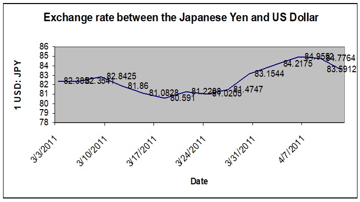
Data and graph showing the exchange rate between the Japanese Yen and US Dollar the month after the earthquake.

Raw data

• March 1: 1 USD = 81.923 JPY
• March 3: 1 USD = 82.385 JPY
• March 9: 1 USD = 82.8425 JPY
• March 12: 1 USD = 81.86 JPY
• March 15: 1 USD = 81.0828 JPY
• March 18: 1 USD = 80.591 JPY
• March 21: 1 USD = 81.2208 JPY
• March 24: 1 USD = 81.0205 JPY
• March 27: 1 USD = 81.4747 JPY
• March 30: 1 USD = 83.1544 JPY
• April 3: 1 USD = 84.2175 JPY
• April 6: 1 USD = 84.9552 JPY
• April 9: 1 USD = 84.7764 JPY
• April 12: 1 USD = 83.5912 JPY

The graph shows how much the Japanese Yen exchanged for 1 US Dollar between March 3, 2011, and April 12, 2011. Following the earthquake and tsunami that hit Japan on March 11, 2011, the Japanese Yen appreciated against the dollar in the week immediately after the disasters. The Yen was strongest on the 18^th of March, hitting the 80.591 marks. The Yen remained strong until the end of March when it began to depreciate.

The significant appreciation of the Japanese Yen immediately after the earthquake and tsunami disasters was unexpected because any major catastrophe of such magnitude is expected to hurt the domestic currency. However, the appreciation of the Japanese Yen is attributed to the actions of Japanese investors immediately after the disasters. Japanese investors invest their money in overseas markets such as the Australian and New Zealand markets due to the higher returns of their currencies. The disaster, however, could have forced the Japanese investors to purchase their Yen back to help with the reconstruction of Japan. Thus, higher demand for the Japanese Yen vis-à-vis a lower demand for foreign currencies such as the US dollar may have pushed the value of the Yen upwards (Honohan, 2007).

The depreciation of the Japanese Yen beginning at end of March may have been caused by several factors. First and foremost, Japan is a net exporter, particularly of electrical and electronic goods. Therefore, a stronger Yen hurts Japan’s exports because it makes Japanese goods more expensive to foreigners but foreign goods cheaper to the Japanese (Honohan, 2007). This could hurt the Japanese economy and could further deteriorate the economy, which had already been weakened by the earthquake disaster. To avoid this, the Central Bank of Japan (BOJ) was forced to intervene by lowering the value of the Japanese Yen against major foreign currencies such as the US dollar. Hence, an interventionist policy by the monetary authority is another factor that influenced the exchange rate between the Japanese Yen and the US dollar following the earthquake.

Rules versus discretion

The rule versus discretion is one of the oldest debates, central to monetary economic policy. Under a rules-based approach to monetary policymaking, there is a predefined reaction function that specifies the adjustment of policy to changes in certain variables. On the other hand, under the discretion-based approach, policy decisions are made on an ad hoc, that is, according to the current evaluation of policy needs. Although the extent of activism is substantially smaller under a rules-based approach (it is limited to pre-determined, state-contingent policy changes), in essence, both systems can be considered as an activist in nature. The unique characteristic between the rules approach and the discretion approach is how the monetary authority decides to set policy in the future (Aerdt & Houben, 2000).

In the United States, the nature of the monetary policy is discretionary. The monetary authority in the U.S. is the Federal Reserve, which has unlimited capacity to influence the monetary policy. In particular, the Federal Reserve alters existing policy or makes new policy in response to the economic events in the country, and especially if there are adverse shocks. For instance, the Fed has reacted when there is high inflation in the country. It has also responded on several occasions to economic or financial crises in the country, such as the stock market crash, sub-prime mortgage crisis, and the negative effects of the September 11, 2001, terrorist attacks.

The arguments made in favor of a rules-based approach are based on the claim that discretionary policymaking has a high likelihood of destabilizing the economy. This is because policymakers lack complete and perfect information about the economy and therefore, any measures undertaken will be ill-timed. When policy-making is discretionary, the public at large is unable to envisage future policies, thereby increasing uncertainty. Also, because of the high degree of freedom granted to policymakers, the concerned authorities may prioritize short-term goals or personal interests over long-term goals and the interests of the society at large, thus deteriorating the entire economic development in the medium term. The supremacy of rules is thus seen to reflect the limited understanding of the policy transmission process, the role of policy predictability in stabilizing expectations, the tendency of the private sector to revert swiftly to equilibrium, and the inappropriate prioritization that results from the unavoidable incentives to boost short-term economic activity or increase fiscal revenues (Aerdt & Houben, 2000).

Opponents of the rules-based approach, on the other hand, base their arguments on the lack of steady relationships in the economy and on the necessity of maintaining policy flexibility for curtailing the adverse consequences of future unexpected developments. Monetary authorities under a discretionary policy system therefore have the benefit of being able to take into account the unfolding developments when they decide on the policy position towards their medium-term goals. Because the authorities will act to counteract the destabilizing consequences of unexpected events, economic agents will face less aggregate uncertainty under a discretionary policy than under a rules-based policy (Aerdt & Houben, 2000, p. 38).

Economy stagnation

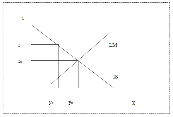
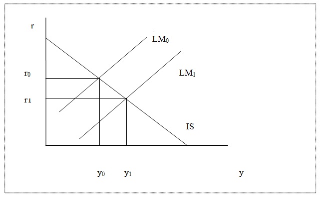
A negative oil shock leads to high prices of commodities (inflation) as well as unemployment as the economy stagnates. The occurrence of inflation and unemployment at the same time is referred to as stagflation. Stagflation goes against the Philips’ curve which postulated that there is an inverse relationship between inflation and unemployment such that a high inflation rate is associated with a low unemployment rate and a low inflation rate is associated with a high unemployment rate. The intervention policies gave and their effects can be illustrated in the diagrams below:

The graph shows the interaction between the IS and the LM curves. The IS curve shows the equilibrium in the product market, while the LM curve shows the equilibrium in the money market. The horizontal axis shows different levels of output in the economy, while the vertical axis shows different levels of interest rates. The initial equilibrium is the point at which the LM and the IS curves intersect, giving the equilibrium output level of y₀ and the equilibrium interest rate level of r₀. If the interest rate is raised, say to r₁, it would have a positive effect of reducing the level of prices in the economy. This is because high-interest rates increase the cost of borrowing which in turn reduces the demand for goods and services. A fall in aggregate demand reduces the level of inflation in the economy. On the other hand, a rise in the interest rate will lead to a decrease in the output level from y₀ to y1. With low output levels, firms would be forced to lay off workers and machines, leading to a high unemployment rate (Moomaw, Olson & McLean, 2009). A further and consistent fall in output and employment rates may lead to a deep recession.

The graph indicates the interaction between the IS and the LM curves. At the initial equilibrium, the equilibrium level of output is y₀ while the equilibrium interest rate is r₀. An expansionary monetary policy, for instance, an increase in the level of money supply in the economy will shift the LM curve outwards from LM₀ to LM₁. This will have two direct effects. First, the level of output in the economy will increase from y₀ to y₁. This implies that the employment level will also increase as firms will hire more labor and machines to achieve a high output level. Second, the interest rate will fall from r₀ to r₁. A low-interest rate will reduce the cost of borrowing and as a result, people will borrow and demand more goods and services. The increase in demand for goods and services will push the level of prices upwards thereby causing inflation (Sidlow & Henschen, 2008). The two graphs show that the consequences of a negative oil shock cannot be curtailed using one policy. Rather, it requires a combination of policies, both fiscal and monetary, working at the same time, to address both the problem of inflation and unemployment.

Saving

The marginal propensity to save is the fraction of income that is spent on savings (Young & Zilberfab, 2000). An increase in the marginal propensity to save may come about if people have expectations of a near economic downturn that may result in lower wages and higher unemployment levels. If the fraction of income spent on saving increases, it means that savings will be greater than investment, for all the combinations of interest rates and incomes. Hence, the equilibrium in the IS curve will be distorted. As a result, the leakage will be more than the injection, thus leading to a fall in the income level until the level of savings equals the level of investment.

When people save more and spend less, the effect is a fall in the aggregate income such that the lower-income multiplied by the higher fraction saved results in the same total savings, which is equal to the unchanged level of investment. As a result, every level of interest rate will be associated with a lower level of income in the new IS than in the initial one (Gamber & Colander, 2006). The IS curve will shift to the left. The new intersection with the LM curve will take place at a lower interest rate and a lower income level than previously. An increase in the marginal propensity to save will therefore lead to a fall in national income and a fall in the interest rate.

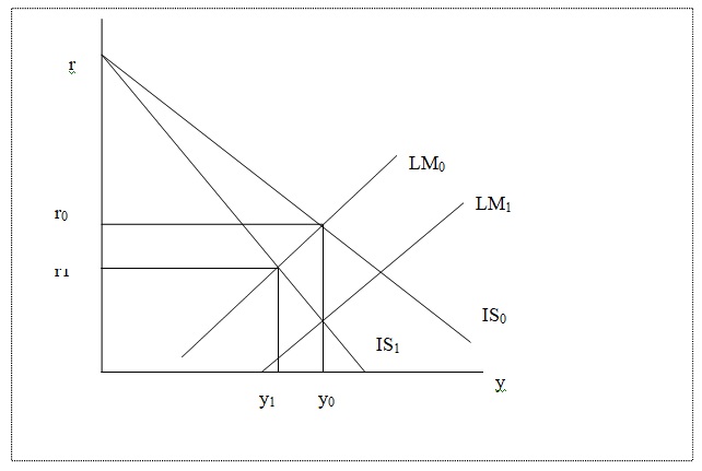
The graph shows the intersection of the LM and IS curves for different combinations of interest rate and income (output) levels. The initial equilibrium point is given at the point where the LM curve intersects with the IS₀ curve, giving an equilibrium level of income (output), y₀, and interest rate, r₀. When the marginal propensity to save increases, the IS curve pivots to the left to IS₁, (that is, it rotates around the original IS curve, IS₀) giving new equilibrium levels of income (output), y₁ and interest rate, r₁, which are lower than the initial equilibrium levels. The lower output level translates into lower employment levels as firms lay off workers and machines. Also, a lower output level implies there is a recession in the country, at least in the short run. The fiscal budget will also be negatively affected by a reduced level of output.

The lower interest rate on the other hand causes a high inflation level because it reduces the cost of borrowing which in turn increases the demand for goods and services, thereby pushing the level of prices upwards. Similarly, an increase in the marginal propensity to save will increase the level of investment in the country. This is because a higher marginal propensity to save reduces the level of interest rates, which in turn encourages investment in the country (Gamber & Colander, 2006).

To restore the economy to its original output level, the monetary authority can implement an expansionary monetary policy, which will work by shifting the LM curve outwards to LM1. The output level will move back to y₀ but the interest rate will fall further to be equal to the increase in the savings level.

References

Aerdt, C. & Houben, J. 2000. The evolution of monetary policy strategies in Europe. London: Springer.

The exchange rate between the Japanese Yen and the US Dollar. Web.

Gamber, E. & Colander, D., 2006. Macroeconomics. Cape Town: Pearson South Africa.

Honohan, P., 2007. Dollarization and exchange rate fluctuations. Geneva: World Bank.

Moomaw, R. Olson, K. & McLean, W., 2009. Economics and contemporary issues. Mason, OH: Cengage Learning.

Sidlow, E. & Henschen, B., 2008. America at odds. Mason, OH: Cengage Learning.

Young, W. & Zilberfab, B., 2000. IS-LM and modern macroeconomics. London: Springer.