Introduction
To begin with, it should be stated that the economic theory and math have been developing separately for the last 20 years, nevertheless, the central principles of math functions and calculations stayed the same, and the aim of this paper is to consider these principles and compare the math functions with the economic calculation techniques and make the parallels.
The actual value of this work is covered in the notion that the analysis of the similarity of the techniques and rules of math and economic calculation will help to foster the further development of math functions, applicable for the economic theory. The fact is that the central branch of the economic analysis from the math perspective was the probability theory and the stochastic analysis.
Originally, the development of economic theory in these directions caused important progress in the sphere of pricing theory and interest-rate modeling. The paper will be aimed at regarding various directions of the economic theory and applying the notions of this theory to math principles, including inverse functions, functions of two or more independent variables, curvilinear functions, and linear functions. The linkage between one function and one economic concept will be explained.
General Review of the Economic Approaches in Calculations
First, it should be emphasized that the math functions in economics are generally intended for the performance of the decision-making process by the means of complex calculations, for guarantying the high precision and accuracy of the decision-making process. The fact is that the approaches, which are generally regarded in the financial literature do not fully represent the economic image of the world, and economic literature typically pays less attention to the high-level quantitative approach. In the light of this perspective, it should be emphasized that the quantitative methods, which are of particular importance for the economists were developed by the mathematicians, and stay available for an essentially restricted audience, while these approaches could become the bridges of math and economics.
The math functions, which are generally used for the economic calculations and decision-making process are related to the consumption functions, and help to realize the issue of “What is going wrong in economics”. Metzler (2001, p. 907) emphasizes the following statement on this perspective:
The math functions have the merit of relative simplicity: the economic thinking behind them can be understood. In the more “advanced” realms of mathematical economics, can be found with equations with literally hundreds of variables, coefficients, and constants, all of them vague and slippery and open to serious debate. The whole thing reaches its acme in the so-called “game theory” balderdash. Here math usurps economics altogether, with pernicious results. The equations and the algorithms, which the myopic game theorists cook up, serve only to give economists and bureaucrats the comforting illusion that they know what they are doing.
Principles of Applying Math Functions to Economic Problems
Generally speaking, the math functions are regarded as the basic calculations of the economic models. Depending on the nature of the economic environment and the principles, which are modeled, these models may be stochastic or non-stochastic and discrete or continuous. The practical level of math analysis requires quantitative modeling, which involves several independent methodologies, which depend on the previously listed natures of the economic environment.
Stochastic Models
These models are intended for modeling the values, which are openly observable over the time period, which is considered in the model. Originally, these are statistical curvilinear and linear models, which are used for formulating and testing hypotheses on the matters of the economic processes and estimating the required parameters for these processes.
Non-Stochastic Mathematical Models
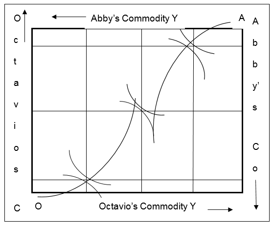
These models may be either qualitative (if used for modeling the social choice perspective of the economic principles) or quantitative (rationalization of financial variables). These are the hyperbolic variables, and these are mainly represented by the curvilinear functions and functions with two or more independent variables. These models generally presuppose the usage of two-dimensional graphs, such as Edgeworth box
Qualitative Models
These are either discrete or continuous, depending on the scales of the modeling and the economic level of the principles applied. It should be stated that qualitative models are subjected to the lack of precision because of resorting to the macro-economic principles.
Math Functions in Economics
Taking into consideration that the probability theory in economics and the game theory approach is the origination of the Austrian school of economics, some researchers (Colander, 2004; McGregor, 2001) emphasize the statement that the integration of math and economics allows politicians to socialize the financial activities of the population.
The most universal function of math functions in economics is the capability of optimization. While optimization in any sphere is regarded to be the selection of the best element from the available alternatives, math functions are intended for searching this alternative and applying the gained results for the economic principles. In other words, this means the solving of a problem, where minimization or maximization of a real function is required. The values for such solving are selected systematically from the set of economic values and variables, while the values may be either real or integer. Lawler (2004, p. 740) gives the following explanation for this statement:
This formulation, using a scalar, real-valued objective function, is probably the simplest example; the generalization of optimization theory and techniques to other formulations comprises a large area of applied mathematics. More generally, it means finding “best available” values of some objective function given a defined domain, including a variety of different types of objective functions and different types of domains.
The best available value, in this perspective, maybe regarded through the math expression, which is generally used for optimization.
Thus, there is a function f, where A → R from some set A to the real numbers.
An element x0 in A such that f(x0) ≤ f(x) which is represented as x in A (“minimization”) or such that f(x0) ≥ f(x) for all x in A (“maximization”) requires to be found. (Earley, Seltzer, Boulding, 2001, p. 120)
Originally, this formulation is called an optimization problem and is the matter of linear functions. In accordance with the Review of Fundamental Mathematics, any linear relation between y and x can be expressed in the algebraic form:
y = a +bx
where y is the dependent variable, x is the independent variable, a is the intercept parameter, and b is the slope parameter. The terms a and b are called parameters, rather than variables because their values do not change along with the graph of a specific linear function. The intercept parameter, a, gives the value of y when x = 0. For the line representing y = f (x), when x = 0 the line crosses the y-axis. Hence the name “intercept” parameter.
The fact is that numerous theoretical problems may be modeled and solved with the assistance of the optimization strategy, which is intended to use the linear math functions. This framework allows to formulate the problems in the sphere of economy regarding the perspective of the expenses minimization, making this minimization properly grounded with the help of math, thus the f functions may represent the expenses of the modeled system.
From the position of this perspective, it should be emphasized that the function itself is represented in the A meaning, which is specified by a set of restraints in the subset of the Euclidean space Rn, where equalities and inequalities of the A range will satisfy the given range. As it is stated in Kristol (2002), the A domain of these functions is regarded to the choice set, while the elements of the whole range are the candidate solutions. He also emphasizes the following:
The function f is called, variously, an objective function, cost function, energy function, or energy functional. A feasible solution that minimizes (or maximizes, if that is the goal) the objective function is called an optimal solution. (Kristol, 2002, p. 314)
Reaction Function

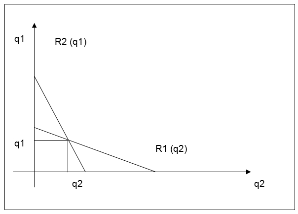
Originally, this function represents the equilibrium quantities in the context of a solution to two reaction functions in Cournot duopoly. Every function is expressed as a linear equation, which depends on the quantity demanded. The slope of the line, required for the precise economic solution of the problem, expressed by this function, represents the function y = f (x), and in accordance with this function, it is defined as the change in the dependent variable y divided by the change in the independent variable x:

where the △ symbol indicates the change in a variable. When y is plotted on the vertical axis and x is plotted on the horizontal axis, the change is y can be called rise, the change in x can be called run, so the slope of the line is frequently referred to as rise over run. In Figure A.1, moving from the top of the line where it intersects the q axis down to the bottom of the line where it intersects the p axis, the rise is -100 (=△q). The run is +50 (△p), and so the slope is -2.
Thus, the linear elements of economic theory such as supply/demand, quality/quantity, and other linear variables may be defined by this function.
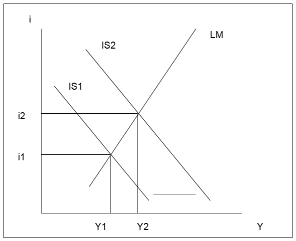
Another example of the linear functions is represented in the Keynesian macroeconomic model. The fact is that it is a classical economic approach, which is intended to forecast the intersection of “real” economic activity, considering such factors as spending, income, savings rates. Moreover, the aim of this approach is to calculate the matters of the decisions made in the financial markets: Money supply and Liquidity preference. Originally, this model is not used widely; nevertheless, it gives the basic image of the macroeconomic processes.
The graphic representation of this math function is the following:

When the Investment Saving (IS) curve moves to the right, thus increasing the interest rates (i), thus, the economic factors grow. Originally, it is the basic theoretical representation of the GDP rates (Y). This function can not be applied for microeconomic principles, or the economic relations of the individuals, as Keynesian economic principles may be related only to macro-economic principles, and represent the monetary policies, the allover economic trends. As Stigler and Friedland (2005, p, 339) emphasize:
A shift in the IS or LM curve will cause a change in expectations, causing the other curve to shift. Most modern macroeconomists see the IS/LM model as being at best a first approximation for understanding the real world.
Edgeworth Box

An Edgeworth box is intended to express the contract curve, which is actual for the economic relations with two participants. It is referred to as the central economic concept of the economic principle when all the actions are performed with the consideration of the particular advantage. Originally, this concept was introduced by Francis Ysidro Edgeworth as a math element in 1881 but later was applied in the economy for defining the principles of economic behavior thus, permitting the outcome of each decision to be converted into a change in utility (Udehn, 2002). With the help of this assumption, Edgeworth managed to create the exchange model, which was built on three basic assumptions:
- Individuals, who participate in economic relations act to maximize the utility of the overall economic relations
- Individuals who are interested in their own advantages
- Individuals who are free to deal with any other person independently of any third party, involved in the economic relations.
- In the light of this perspective, this may be also regarded as the function of two independent variables.
This box is an example of the curvilinear function which entails y = a + bx +cx², y = sin x, y = ln x, and t = ex. The slope of a curve varies continuously with movements along the curve. It is useful in studying decision-making to be able to measure the slope of a curve at any one point of interest along the curve. The slope of a curve at the point of tangency is equal to the slope of the tangent line itself.
Thus, from the perspective of the three assumptions by Edgeworth, the financial advantage and benefits of the parties may be calculated. Nevertheless, the total sum should be considered, for the frames of the calculations were known.
As for the inverse functions, it should be emphasized that these are not applicable to relevant economic models, and the models, which resort to these functions are not required in economic practice (Sutter and Pjesky, 2007)
Economic Principles in Math
There is a strong necessity to emphasize that most part of the classical economic principles may be represented by the means of simple geometric rules or math notations. The mathematical part of the economics resorts to the matrix algebraic principles, which the economic analysis tools are based on, for providing the necessary assessment principles, as economic analysis would be impossible without these math tools. Thus, as Metzler (2001, p, 909) claims, the complexity of the economic problems depends on the approach, which is used for loving any particular problem:
Economic problems often involve so many variables that mathematics is the only practical way of attacking and solving them. Alfred Marshall argued that every economic problem which can be quantified, analytically expressed and solved, should be treated by means of mathematical work. Economics has become increasingly dependent on mathematical methods and the mathematical tools it employs have become more sophisticated. As a result, mathematics has become considerably more important to professionals in economics and finance. (Metzler, 2001, p, 909)
In the light of this perspective, it should be emphasized that the attraction of mathematicians for solving the economic problems and outlining the key principles is required for the simplified solving of the practical economics-related issues, while numerous economic problems are often classified as integrated into the scope of applied math. As for the matters of such integration Maurice and Thomas (2008) state that it is generally regarded as a result of the formulation of the economic issues as the issues of the particular economic models, which presuppose the falsifiable predictions in the context of clear assumption of the model itself, thus, creating the new approach for solving economic problems by mathematical modeling. This modeling is explained in detail in Adam Smith’s “The Wealth of Nations” (Colander, 2004)
Conclusion
Finally, it should be stated that the math functions in relation to the economic principles are regarded to be useful for economic modeling, while the practical application of the math principles in economics is useful only for the theoretical grounding of practical models.
The functions, which are represented in the models, described in the paper are the linear, curvilinear, and functions of two or more independent variables. Inverse functions are almost not applicable in the economy, as the models, which are based on these functions are not used in the relevant economic theories, and are not required for economic practice.
References
Colander, David C. (2004). “The Strange Persistence of the IS-LM Model”. History of Political Economy. Duke University Press.
Earley, J. S., Seltzer, L. H., Boulding, K. E., & Gruchy, A. G. (2001). Economic Theory in Review (C. C. Lawrence, Ed.). Bloomington: Indiana University.
Kristol, D. B. (Ed.). (2002). The Crisis in Economic Theory. New York: Basic Books.
Lawler, J. J. (2004). Not Just for the Money: an Economic Theory of Personal Motivation. Personnel Psychology, 51(3), 740.
McGregor, S. L. (2001). Reinterpreting Economic Theory in a Global Reality. Journal of Family and Consumer Sciences, 90(3), 35.
Maurice, S., & Thomas, C. (2008) Managerial economics New York, NY: McGraw-Hill.
Metzler, Lloyd (2001). “Review of Foundations of Economic Analysis”. American Economic Review 38 (5): 905–910.
Quick Fixes, Test Scores, and the Global Economy: Myths That Continue to Confound Us. (2008). Childhood Education, 85(1), 65.
Stigler, G. J. Friedland, C (2005). “The Journals of Economics”. The Journal of Political Economy (The University of Chicago Press) 103 (2): 339.
Sutter, Daniel and Rex Pjesky. (2007) “Where Would Adam Smith Publish Today?: The Near Absence of Math-free Research in Top Journals”.
Udehn, L. (2002). The Limits of Public Choice: A Sociological Critique of the Economic Theory of Politics. New York: Routledge.