The population of interest in this article
For this article, the population of interest is the people who suffer from obesity. The adult population is also dwelled upon, but the research was primarily concerned with obese children and the way their body mass and other health indices developed over years (Kolata 1). It can be concluded that the population that the article focuses upon is mostly obese children of different age.
The sample size
The sample size is 7,738 children of both genders and different races and ethnicities that would be able to represent the entire nation (Kolata 2). The only information that was available concerning the life of children before kindergarten was their birth weights, but they had been closely monitored since their kindergarten age and until they finished the eighth grade. The sample was split between two studies: the first one involved 1,704 children of the Southwest schools, and the second one monitored 5,106 kids from “96 schools in California, Louisiana, Minnesota and Texas” (Kolata 3).
The article states that “When the children entered kindergarten, 12.4 percent were obese — defined as having a body mass index at or above the 95th percentile — and 14.9 percent were overweight, with a B.M.I. at or above the 85th percentile. “ Is 12.4 percent mentioned here a population, a parameter, a sample, or a statistic?
The 12.4 percent data is a piece of statistics since it reflects the part of the studied sample, which represents the whole population. This part of the sample was characterized by a particular parameter (obesity).
The variable of interest. Analysis of the main focus of the study according to the article
Technically, there are two variables in the study. The body mass index (BMI, which is used to define the level of obesity in children) is the focus of the article, and the research that is described in it is aimed at determining this variable. However, the article discusses the changes that occur in an obese person since very young age and until adolescence. Therefore, the researchers demonstrate the changes in the BMI variable with time. This means that BMI is the dependent variable, the changes of which are correlated to and conditioned by the changes in the independent variable, age. As a result, the study and the article are aimed at defining the correlation between age and excessive BMI, and they succeed in determining that overweight children tend to remain overweight or grow heavier to the point of obesity with age. “The main message is that obesity is established very early in life, and that it basically tracks through adolescence to adulthood” (Kolata 1).
In terms of the target population, what branch of statistics is being practiced?
In this case, we will be practicing inferential statistics because the study sample that amounts to 7,738 children is created to represent the entire population of obese people of particular age and is used to make a conclusion about the latter as a whole. Naturally, the population is much larger than the sample, but the characteristics of the sample are chosen in a way that would allow inferring the properties of the entire population (Spatz 3).
A study by researchers from Columbia University and Mount Sinai Medical Center in New York, used data from a wide-ranging survey of the behavior of children in New York. The study, which tracked a number of adolescents into adulthood, found that young people watching one to three hours of television daily were almost four times more likely to commit violent and aggressive acts later in life than those who watched less than an hour of TV a day. 0.0085 % of the people who lived in New York participated in this survey and the children and their parents were periodically interviewed about TV habits, violence and aggression. The authors found that 5.7% of the survey participants who reported watching TV for eight hours daily as adolescents, which was 40 people, committed aggressive acts against others in subsequent years and that was the most frequent answer. Those aggressive acts included threats, assaults, fights, robbery and using a weapon to commit a crime. The remaining survey participants reported watching a sum of 3014 hours. The standard deviation for the TV watching time was 1 hour and 2 minutes.
The population size in this example
Since 5.7% of the participants amounted to 40 people, the study sample equaled 100∕5.7×40= 701 people.
This means that 701 people are 0.0085% of the population; therefore, the population size of the example amounts to 8,247,058 people.
The sample mode in this example
8 hours was the sample mode because it was the most frequent answer.
What is the sample mean in this example?
8×40 hours +3014=3334
3334÷701=4.75 hours
The calculations above are explained as follows: 40 people watch TV 8 hours a day while the rest of the sample reported the sum of 3014 hours. The sample mean requires adding the two numbers and dividing them by the number of the people involved (701). The sample mean equals 4.75 hours.
If this distribution is bell shaped, what is the lower and upper bound of hours for 95 percent of participants to watch TV?
95% falls within the second standard deviation from the mean in a bell-shaped distribution curve. This means that the boundaries will be 4h 45 minutes +/- 2h 4min. When worked out, these values give 6h 49 min for the upper boundary and 2h 41 min for the lower boundary.
Dataset Xr02-33. NY Times reports that around 90 percent of American households buy ready-to-eat breakfast cereal, which remains the largest category of breakfast food with some $10 billion in sales as of last year. With this large of a market, cereal production companies often need to know more about who is buying their product. The marketing manager of a major company wanted to analyze the cereal sales among college and university students who eat breakfast cereal. A random sample of 285 students was asked to report which of the following is their favorite cereal:
- Kellogg’s Raisin Bran
- Kellogg’s Frosted Mini Wheats
- Kellogg’s Special K
- GM Cinnamon Toast Crunch
- GM Cheerios
- Post Honey Bunches of Oats
- Other brands
The responses were recorded using the codes 1, 2, 3, 4, 5, 6, and 7, respectively. Use a graphical and tabular method to summarize these data. What can you conclude from the chart? Also the gender of the respondents was recorded as 1 for males and 2 for females. Use a graphical technique to determine whether the choice of cereal differs between genders.


From the summarized data it is obvious that the most popular cereals are Kellogg’s Raisin Bran followed by Kellogg’s Special K and Cheerios. The least popular of the presented brands is the GM Cinnamon Toast Crunch.
There are similarities and differences in the choice of cereals of people of different genders that can be clearly seen in the graph. The preference of RB and C is higher among females than males. On the other hand, males took a greater liking to FMW, FK and CTC. The tastes of females and males do not differ too much for most cereals with the exception of C and FK. It can be concluded that C is the least favored of the top three brands among men; females, on the other hand, prefer it over FK. Also, CTC is the cereal that is favored the least both by males and females.
Dataset Xr02-54. A survey of the business school graduates undertaken by a university placement office asked, among other questions, the area in which each person was employed. The areas of employment are:
- Finance
- Accounting
- Marketing
- Economics
- Other
The responses were recorded using the codes 1, 2, 3, 4 and 5, respectively. Additional questions were asked and the responses were recorded in the following way.
Do female and male graduates differ in their areas of employment? If so, how?

From the graph, it is evident that most areas of employment have uneven numbers of females and males (with the exception of marketing). The differences are especially visible in three of the fields: ladies are mostly employed in finance and economics while gentlemen prefer accounting. Also, the “other” category includes more males than females, but it is also the smallest group.
Are area of employment and job satisfaction related?
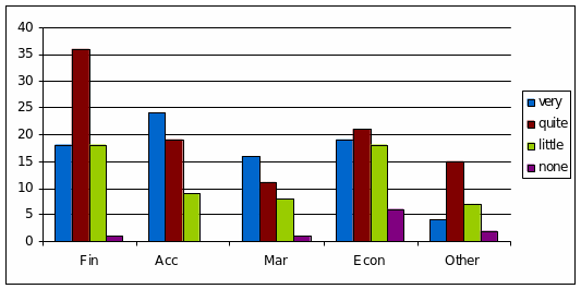
The graph shows that areas of employment and the level of job satisfaction can be related, and certain tendencies can be found. In particular, the field of accounting has the greatest rates of very satisfied people while the largest part of the employees of the finance area reported being relatively happy with their job (quite satisfied). At the same the time, the rates of relative dissatisfaction was the highest for finance and economics as well. Apart from that, the employees of the area of economics reported the highest level of dissatisfaction with their job (no satisfaction at all). It should be pointed out that finance and economics also employ the greatest numbers of people. This could explain the differences in their satisfaction. In general, people working in areas of accounting and marketing report less dissatisfaction with their jobs than those in finance and economics (Greenstein 39).
Dataset Xr03-76. To determine car insurance premiums, companies must have an understanding of the variables that affect whether a driver will have an accident. The age of the driver may top the list of variables. The data file Xr03-76 lists the number of drivers in the United States, the number of fatal accidents, and the number of total accidents in each age group in 2002.
Calculate the accident rate (per driver) and the fatal accident rate (per 1,000 drivers) for each age group.
Graphically show the relationship between the ages of drivers, their accident rates, and their fatal accident rates (per 1,000 drivers).
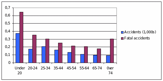
Interpretation of the findings.
The graph shows that the rates of both accidents and fatal accidents tend to decrease as the driver’s age increases. However, when the driver’s age goes beyond 74 years, he or she is more likely to cause a fatal accident. The increase is rather sharp when contrasted with the previous age group; this figure is comparable to that of the number of fatal accidents caused by the drivers in the age group of 25-34 (Gibaldi 23). Also, the contrast between the numbers of fatal accidents caused by the youngest drivers and those belonging to the next age group is very impressive: the figure decreases almost in half. The numbers of fatal accidents exceed those of simple accidents for every age group.
6. Dataset Xr04-17. In an effort to slow drivers, traffic engineers painted a solid line 3 feet from the curb over the entire length of a road and filled the space with diagonal lines. The lines made the road look narrower. A sample of car speeds was taken after the lines were drawn.
Calculate the mean, median, and mode of these data.
Description of the information acquired from each statistic calculated in part (a).
The cars travelled at a mean speed of 32.908 meters per hour. At the same time, the cars mostly drove at the speed of 32mph since this was the speed that appeared most often on the record (this is the mode). In this situation, the median is the same number; therefore, half of the cars travelled at a speed below 32mph and the other half exceeded this number (Graziano and Raulin 57).
7. Dataset Xr04-36. Waiting lines or queues are important parts of our everyday life. For example, we wait in line at a supermarket, such as Carrefour or Co-op to go through the checkout counter. There are two factors that determine how long the queue becomes. One is the speed of service. The other is the number of arrivals at the checkout counter. The mean number of arrivals is an important number, but so is the standard deviation. Suppose that a consultant for the supermarket counts the number of arrivals per hour during a sample of 150 hours.
Calculate the standard deviation of the number of arrivals.
The mean number of arrivals at the supermarket is 98 and the standard deviation is 15.
Assuming that the histogram is bell shaped, interpret the standard deviation.
In this case, the standard deviation allows defining the range of the typical number of arrivals and its correlation with hours (Spatz 58). For example, in 68% of the hours the number of arrivals ranges between 83 and 113, in 95% of the hours – between 68 and 128, and in 99.7% of the hours – between 53 and 143 (Bax 43). The greater is the percentage of the hours that is considered, the greater is the range of the number of arrivals. This is explained by (and explains) the bell shape of the histogram.
Suppose that you bought a stock 6 years ago at $6.The stock’s price at the end of each year is shown here.
Rate of return for the first year= 5-6/6=0.1667
Rate of return for the second year=7-5/5=0.4
Rate of return for the third year=7.5-7/7 = 0.0714
Rate of return for the fourth year= 11 – 7.5/7.5 =0.4667
Rate of return for the fifth year= 15-11/11 = 0.3636
Rate of return for the sixth year= 12.5 – 15 / 15 = -0.1667
Average and median rate of return
Median = (0.07 + 0.36)/2 = 0.215

Compound rate of return


– 1=0.129
The geometric mean is the most appropriate part of the statistics as it gives a projection of the investment to be made in the next 6 years, that is, defines its future value: 5*(1.129)6=12.49 (12.5) (Asadoorian and Kantarelis 22).
For each of the following types of data, determine the type – either interval, ordinal, or nominal.
The weekly closing stock price of Google – interval: the “intervals between the numbers are equal,” that is, a week (Spatz 11).
- Occupation – the numbers here are used as names without a “real quantitative value” (Spatz 10).
- Yearly education level – interval as it deals with the interval of a year.
- The list of movies that received an Oscar last year –- nominal, no quantitative value.
- Rating of a movie on IMDB using stars – ordinal: places the movies in order of one being “greater” than the other (Spatz 10).
- Eye color (blue, brown, green, hazel) of all AUS students – nominal, no quantitative value.
- Type of cancer for the patients in the UAE hospitals – nominal, no quantitative value. Unless stages of cancer are implied, then it can be considered ordinal.
- The degree you obtain – nominal, no quantitative value.
- Models of a car (i.e. Toyota Camry, Corolla, Rav4, Land Cruiser) – most often nominal, unless a part of the model’s name implies the order in which it appeared (for example, Toyota Camry XV10 and XV20); then it can be considered ordinal.
- Pulse rate of a patient having a heart attack – interval: measurements of the pulse rate are aimed at defining the frequency of the impulses; the pulse rate, therefore, is a piece of interval data.
Data from the last statistics course was collected on the weekly number of hours each student studied and their grade on the final for three students. Calculate the sample variance, sample standard deviation, sample covariance, and sample coefficient of correlation (without the help of a computer software) for the following data and show your work
Works Cited
Asadoorian, Malcolm O, and Demetrius Kantarelis. Essentials of Inferential Statistics. Lanham: University Press of America, 2005. Print.
Bax, Steve. Cambridge Marketing Handbook. London, U.K.: Kogan Page in association with Cambridge Marketing Press, 2013. Print.
Gibaldi, Joseph. MLA Handbook for Writers of Research Papers. New York: Modern Language Association of America, 2003. Print.
Graziano, Anthony M, and Michael L Raulin. Research Methods. Boston, MA: Allyn and Bacon, 2013. Print.
Greenstein, Theodore N. Methods of Family Research. Thousand Oaks, Calif.: Sage Pulications, 2006. Print.
Kolata, Gina. “Obesity is Found to Gain its Hold in Earliest Years.” New York Times,2014. Web.
Spatz, Chris. Basic Statistics. London, UK: Cengage Learning, 2010. Print.