Market structures
Perfectly competitive markets have a large number of small firms acting independently. In addition, firms produce homogenous products, there is the ease of entry, and all market participants have perfect market information. (Layton, Robinson & Tucker, 2009). On the other hand, monopolistic competition is characterized by a large number of small firms and buyers, differentiated products, free entry and exit, and intensive advertising (Hubbard, Garnett, Lewis & O’Brien, 2010). Lastly, oligopoly market structure is characterized by few but large firms, barriers to market entry or exit, strong mutual interdependencies, aggressive advertising, and undifferentiated (Hubbard, Garnett, Lewis & O’Brien, 2010).
Real-life examples
The cement manufacturing industry in Australia is a good example of an oligopoly market. Companies in this industry include Adelaide Brighton Cement, Cement Australia, and Boral. They produce identical products and come together when making pricing decisions (Cement Industry Federation, 2014). The greengrocer retailers in Sydney, Australia, are good examples of a perfectly competitive market. They offer homogenous products and have no barriers to entry or exit in the market. On the other hand, the soft drinks companies in Australia are monopolistic. These companies include Schweppes, Berts Soft drinks, Coca-Cola, and Lion Pty among more others.
Long-run equilibriums
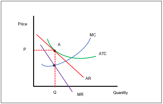
Monopolistic firms make supernormal profits in the short-run. Supernormal profits provide an incentive for new firms to enter the market. As the new entrants continue to enter the market, the quantity supplied increases as the market price decreases. This goes on until the firms start to make normal profits. This is the point where the MC=MR. It is at this point that a monopolistic market is said to have reached its long-run equilibrium. The graph below illustrates the monopolistic market long-run equilibrium (Hubbard, Garnett, Lewis & O’Brien, 2010).
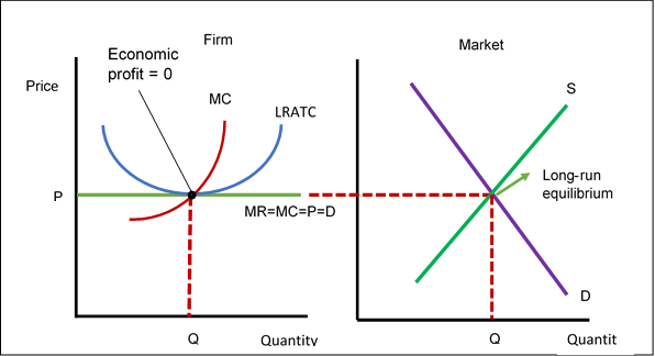
In a perfectly competitive market, economic profits provide an incentive for new firms to enter the market. This causes an increase in the supply of the product in the market. The increased supply causes the market price to fall. The market price falls until the firms in the market start to make economic losses. At this point, the firms are making zero economic profits. In the long-run, the economic losses make the firms to exit the market. This is the point where MR=MC=D=P. The graph below illustrates the long-run equilibrium in a perfectly competitive market. (Hubbard, Garnett, Lewis & O’Brien, 2010).
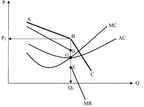
Oligopolistic firms use prices to remain competitive in the market. When a single firm increases its prices, other firms maintain their prices. The demand for goods falls after the prices are increased, and hence affects its revenue. The oligopolistic firms then decrease their prices, causing others to follow suit. An equilibrium quantity and price are achieved at the kink. This is the long-run equilibrium of an oligopolistic market (MR=MC) (Hubbard, Garnett, Lewis & O’Brien, 2010).
Consumer outcome
The monopolistic competition offers the best outcome for consumers. First, it is associated with innovative behaviours (Gillespie, 2013). Firms have to differentiate products to gain a share of the market. The consumer benefits because high-quality products are made available at competitive prices.
Producer outcomes
A perfectly competitive market offers the best outcomes for producers (Gillespie, 2013). The free entry in the market increases the demand for inputs. Producers produce the inputs in mass. In the end, they enjoy the decreased costs of production and increased revenues.
Real GDP components
The net export component is the first real GDP component, which is discussed in the article. According to (Jackson, Mclver & Bajada, 2007), net export refers to the difference between exports and imports of an economy. In 2013, the Italian exports were forecasted to increase by an annual rate of 2.1%. This was anchored on the increase in demand for the Italian goods by the non-EU trade economies. On the other hand, net imports declined by -1% in 2013.
Private consumption is the second component of the real GDP. It refers to the market value of goods and services purchased by households and firms (Jackson, Mclver & Bajada, 2007). The annual percentage change in private consumption in Italy was expected to shrink by -2.0% in 2013 due to the declining household disposable income. Third, public consumption component of real GDP refers to the current and capital spending by a central government. In 2013, the annual percentage change in public consumption in Italy was expected to decline by -2.0% (European Commission, 2013).
The investment component of the real GDP refers to either public (government) or private (households and firms) investment in instruments within an economy (Jackson, Mclver & Bajada, 2007). The investment in Italy was expected to decline in 2013 due to the tight financing conditions that were experienced in the country. The gross capital formation that was projected to decline by -3.0% attributed to a -2.4% decline of equipment investment (European Commission, 2013).
Private and public consumption and investment determine the domestic demand for goods and services. Domestic demand was forecasted to decline by -2.0%. On the other hand, net exports were forecasted to contribute to the annual change in GDP by 0.9%. The aforementioned components resulted in -0.1% annual change in GDP.
AD/AS model
Model explanation
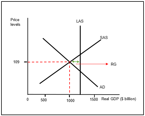
The model above represents a full-employment equilibrium of the Italian economy (Jackson, McLver, McConnell & Brue, 2007). The equilibrium price level is $109 billion, and the real GDP is $1000. On the other hand, the potential GDP is $1150 billion. The real GDP is less than the potential GDP. This results in a recessionary gap of $150 billion.
Fiscal policy
There will be an excess supply of labour in the economy if a fiscal policy is not pursued. This will lead to unemployment and a decline in costs and wages. To address this problem, expansionary fiscal policy tools such as transfer payments, taxes, and government purchasing can be used to close the recessionary gap (Jackson, McLver, McConnell & Brue, 2007). An increase in government purchasing and transfer payment, coupled with tax cuts, will increase disposable income within the economy. This will stimulate consumption, hence shifting the AD to the right.
Self-correction
In the long-run, there will be an economic self-correction to close the recessionary gap. Wages and other production resources will decline (Arnold, 2010). Resource market imbalance will also be eliminated. The short-run AS will increase. The intersection of SRAS, AD, and LRAS will determine the equilibrium point. The economy will be at full employment at this point. The intersection point is the long-run equilibrium. The graph below represents this scenario.
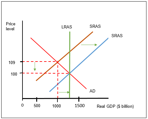
The outcomes of self-correction are good because fiscal or monetary policies can cause business cycles that may be worse than the current situation. In addition, these fiscal or monetary policies may be prone to time and variable lags, and hence destabilize the economy of a country. Therefore, there is no need for monetary or fiscal policies (Arnold, 2010).
List of references
Arnold, RA 2010, Macroeconomics, South Western Cengage Learning, Mason, OH.
Cement Industry Federation 2014, Australia’s Cement Industry. Web.
European Commission 2013, European economic forecast winter 2013, European Economy, No. 1. Web.
Gillespie, A 2013, Business economics, Oxford University Press, London.
Hubbard, RG, Garnett, AM, Lewis, P & O’Brien, AP 2010, Essentials of economics, Pearson, French Forest, Australia.
Jackson, J, Mclver, R, & Bajada, C 2007, Economic principles, McGraw Hill, North Ryde, Australia.
Jackson, J, McLver, R, McConnell, & Brue, S, 2007, Macroeconomics, McGraw Hill, North Ride, Australia.
Layton, AP, Robinson, TJC & Tucker, IB 2009, Economics for today, Cengage Learning, South Melbourne, Australia.