Paired t test
This analyzes the possibility of an improvement in the quality-of-life measure for ten patients taken at random from those who participated in a trial of a minimally invasive procedure to treat Benign Prostatic Hyperplasia (BPH). BPH is a non-cancerous prostate gland enlargement common to millions of elderly men. The two variables in question are qol_base (quality of life at baseline, before treatment) and qol_3mo (the hypothesized improvement after three months of staying with the treatment.
Table 1.
Table 1 (alongside) from the output of the paired samples t test shows, first of all, that mean QoL had “fallen” from 3.80 at baseline to 2.10 after three months. This is a positive finding since QoL was a self-rated scale comprising the items: 0=Delighted, 1=Pleased, 2=Mostly satistifed, 3=Mixed, 4=Mostly dissatisfied, 5=Unhappy, and 6=Terrible.
Table 2.
The derived t value of -3.597 in Table 2 above (ignoring the negative sign owing to the sequence in which the two variables were inserted into the SPSS calculation menu) is so high it bears a significance statistic of p = 0.006. The odds are about 6 in a thousand that such a difference could arise due to chance variation alone. Since this significance result far exceeds the criterion value of α = 0.05, one would have to conclude that BPH patients who received the treatment did experience a subjective improvement.
One-sample t test
Testing the variable delta (delt_qol), which gives the result of the simple calculation qol_3mo minus qol_base, we apply 0 as the test value because the reasonable working hypothesis is that the treatment engenders a perceptible improvement in quality of life ratings.
Table 3.
Table 4.
Table 3 (above) shows, first of all, that the mean QoL Delta value is 1.70, suggesting that the 10 patients typically assigned satisfaction ratings two levels higher after three months on the treatment. Table 4 answers the next question, which is that the derived t value of 3.597 for all delta’s minus the benchmark of zero bears a significance statistic of p = 0.006. Once again, the chance that such a large difference from zero could have occurred due to random variation alone is less than six in a thousand. We conclude yet again that the treatment makes a difference for perceived quality of life.
Are Distributions Normal?
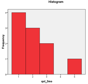
Visual inspection of the histograms alone shows that the QoL ratings at baseline roughly approximates a normal distribution while, three months later, the distribution is decidedly skewed toward the “I’m pleased” end of the scale.
Non-parametric Test of Median
If you have a concern about the small sample size and perhaps non-normal data, choose an appropriate nonparametric test to compare the median QoL score at the baseline and at 3 months. (Hint: You need to research nonparametric tests.)
We employ the nonparametric Wilcoxon Rank-Sum Test to compare the medians of what are nominally two independent groups but really the same group of patients answering rating scales at two points in time.
Since we are testing for a leftward shift in QoL ratings at three months and since the mean rank for all negative deltas outnumber the positive ones (Table 5), the correct usage of the p value reported in Table 6 below is to halve it, thus: p = 0.014/2 = 0.007. As it happens, this is lower than the criterion α = 05.
Table 5.
Table 6.
Even switching to non-parametric statistics yields credence to the same conclusion: BPH patients are subjectively better off after three months under the treatment regiment.
Independent Sample Design
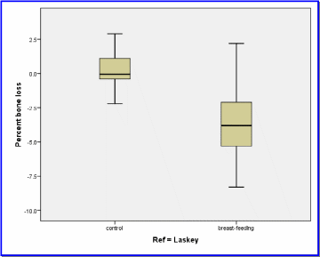
Comparing Boxplots

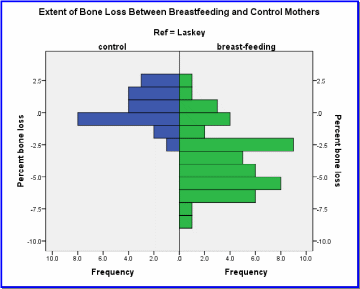
Comparing Histograms

Analysis of Bone Loss Employing a t test
This discretionary test employed the scale variable “change in bone mineral’ density or content and the nominal variable breastfeeding status. Subjects of the study were women who breastfed their newborns and were checked up on at three months of lactation. The control group consisted of formula-feeding mothers and non-pregnant, non- lactating women. Breastfeeding status was used as the grouping variable in the independent-samples t test.
One therefore formulates the hypotheses to be tested as:
H0, the null hypothesis = Among adult women, breastfeeding has no effect on calcium mineral density in bones.
Ha, the alternative hypothesis = Breastfeeding has an effect on bone mineral density in adult women.
Table 7.
Table 8.
Mothers who breastfeed do experience mineral bone loss, as shown by the fact that control women showed an improvement averaging 0.309 on whatever calcium intake they followed (it is not the purpose of the current analysis to account for dietrary and other modifying factors in the Laskey et al. study. The comparable figure for breastfeeding mothers was frank bone mineral loss of 3.59 over the three month run of the study (see Table 7 above). At 3.90, the mean difference in bone mineral change between the two groups lies within the bounds of the 95% confidence interval of the difference (2.8 at the lower bound and 5.0 at the upper limit(Table 8).
A rather high F value for Levene’s Test (11.25, see Table 4) and a test for significance p < 0.05 confirms that the variances in the case-control subject database are homogenous and that one basic assumption of the t test therefore holds. Hence, one scrutinizes the row for “Equal variances assumed”. In either case, the derived t score is high enough for the given degrees of freedom to yield a significance statistic that is below the even more rigorous cut-off of p ≤ 0.01. Since such a difference could have occurred purely by chance less than once in a thousand re-sampling passes, one rejects the null hypothesis, accepts the alternate and concludes that breastfeeding has a deleterious effect on bone mineral density.
95% C.I. for Mean Difference in Percentage of Bone Loss
The 95% confidence interval is shown below.
Table 9.
Cross-Tabulation
Association Between Esophageal Cancer and Alcohol Consumption
This is a test of the relationship between alcohol consumption, measured in grams per day, and the nominal variable with two levels (“no” and “yes”), developing esophageal cancer. The latter was used as the grouping variable in the independent-samples t test.
The hypotheses may therefore be articulated as follows:
One therefore formulates the hypotheses to be tested as:
H0, the null hypothesis = there is no linear relationship at all between alcohol consumption levels and esophageal cancer morbidity. Elevated alcohol consumption is not a predictor of developing esophageal cancer.
Ha, the alternative hypothesis = Adults presenting with a history of elevated alcohol consumption are at greater risk for esophageal cancer.
An exploratory cross-tabulation (Table 10) suggests that those who have not yet developed esophageal cancer are much less likely to be moderate or heavy alcohol drinkers. Nearly half of the control group of 775 adults reported consuming 39 grams a day or less. Nearly all of the remainder, a cumulative 86%, had self-reported alcohol consumption levels of under 80 grams a day.
On the other hand, the 200 men who did develop esophageal cancer tended to cluster around 40 to 100 grams daily. Even more revealing, the distribution skewed towards high consumption.
Table 10.
Both the chi-square and odds ratio tests (Table 11) bore significance statistics with p < 0.001, suggesting that the differences between the case and control groups cannot be accounted for by chance variation.
Table 11.
Table 12.
This is bolstered by the outcome of the independent samples t test (Table 13, below) where, irrespective of the assumption taken about homogeneity of variances across the case and control groups, the t value is so large that, the significance statistic p < 0.001 shows, the difference in alcohol consumption between case and control groups is extremely unlikely to have occurred due to chance alone.
Table 13.
Accordingly, one rejects the null hypothesis and concludes that there is a tangible difference in the propensity of esophageal cancer patients to imbibe more alcohol.
Applicability of Fisher’s Exact Test
Fisher’s exact test of independence across, in this case, the case and control groups of subjects, applies for 2 X 2 contingency tables. This means Fisher’s can be used if the alcohol consumption is recoded as a categorical variable. One would have had to go back to the raw data to reclassify all subjects as either “non-drinker” or “drinker.” Alternatively, a better real-world representation might be “non-drinker or light drinker” versus “moderate or heavy drinker.”
Implementing Fisher’s exact test, the null hypothesis would be articulated as that the relative proportions of the dependent variable, having esophageal cancer, are independent of a second variable. So, the null hypothesis would be articulated around the premise that the proportion who drink (or indulge heavily) is equal among those who contract esophageal cancer and perfectly healthy adults.
Another consideration that voids the applicability of Fisher’s exact test to this data set is that the algorithm is more accurate than the chi-square or the G tests of independence principally when sample sizes are small. In this case, however, the study covered 200 adults in varying stages of esophageal cancer and no les that 775 control subjects. Hence, Fisher’s is not a sound choice in this situation.
Association Between Esophageal Cancer and Alcohol Consumption as Nominal Variable
In fact the database does have a dichotomized version of the alcoholic consumption variable employing 80 grams or more daily as a cut-off for marked indulgence in the vice. The chi-square test is available for testing differences in proportions between categorical variables.
We now test for differences in proportions of those who drink relatively little (if at all) and the heavier drinkers between adults who presented with esophageal cancer or did not.
The hypotheses may be articulated as follows:
H0, the null hypothesis = there is no association between drinking alcohol and esophageal cancer morbidity; put another way, there is no difference in esophageal cancer risk between adults who drink heavily or not.
Ha, the alternative hypothesis = Drinking rate and esophageal cancer are related; esophageal cancer risk is greater for adults who are regular or heavy drinkers.
Table 14.
Crosstabulation reveals that the likelihood of presenting with esophageal cancer is greater when one is a regular or heavy drinker. Just 13.5 % (or one in seven) of light or non-drinkers “came down” with esophageal cancer. With regular or heavy drinking, the risk rose to just under half.
Table 15.
Table 16.
If the proportions of dichotomized drinking rates are representative of the universe of adults, then around eight in ten are light or non-drinkers.
Table 17.
Since the computed chi square statistic of 327.4 and 339.1 for the fact of regular alcohol consumption and esophageal cancer morbidity, respectively, (Table 17) exceeds the criterion chi-square statistic of 3.84 at 1 degree of freedom and α = 0.05, we reject the null hypothesis. As well, the probability of a significant difference like this occurring purely by chance is shown to be less than one in a thousand (p < 0.001). Accordingly, we accept the alternative hypothesis and conclude that adults who drink regularly or heavily bear a higher risk of manifesting esophageal cancer sooner or later.
Manual Calculation of 95% C.I. of Odds Ratio Estimate
The odds ratio can be defined as the ratio of the odds of an event occurring in one group to the odds of it occurring in another group, or to a sample-based estimate of that ratio. These groups might be men and women, an experimental group and a control group, or any other dichotomous classification. If the probabilities of the event in each of the groups are p1 (first group) and p2 (second group), then the odds ratio is:

where qx=1-px. An odds ratio of 1 indicates that the condition or event under study is equally likely in both groups. An odds ratio greater than 1 indicates that the condition or event is more likely in the first group. And an odds ratio less than 1 indicates that the condition or event is less likely in the first group. The odds ratio must be greater than or equal to zero if it is defined. It is undefined if p2q1 equals zero.

