The researcher hypothesized that the time taken to polish a product depended on the size of the product. A linear regression analysis showed that the relationship was significant, F(1)= 54.87, p<.001. There was a strong, positive, linear correlation between the size of the product and the polishing time, r=.70.
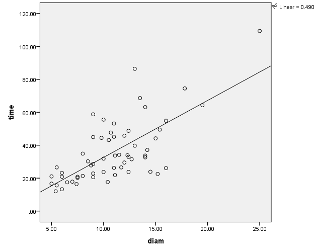
As expected, the time taken to polish a product depended on the size of the product. A scatterplot (shown below) was produced to determine the suitability of the model, where the scatterplot of the two variables showed that a linear model was suitable in this situation.

There is a linear, positive relationship between the time that is spent polishing a product and the size (diameter) of the product, as shown in the scatterplot. It means that one of the assumptions for carrying out a regression analysis has been met.
Although there seem to be some outliers in the scatter plot, they cannot be considered as significant outliers. It implies that the regression equation can predict most of the values; thus, the regression model is sound. The R2 value of 0.49 indicates that 49% variability in time spent in polishing the product can be explained by the diameter of the product.
The Model Summary Table gives two primary values; the R and the R-squared values (Carver & Nash 2012). The R value of.70 shows that there is a strong, linear, positive correlation between the diameter of the product and polishing time. The R-squared value of.49 indicates that 49% variation in the time take to polish the product can be explained by the diameter of the product.
The ANOVA table that is produced in the regression analysis provides values that help in showing how the regression equation fits the data (Johnson & Kuby 2008). In this case, the ANOVA report provides information that helps in showing how well the regression equation predicts the time spent in polishing the product.
The ANOVA report for the time of polishing and the diameter of the product shows that the regression model predicts the time spent on polishing the product significantly well because the F value is significant, p<.05. In other words, the regression model is significance p=.001 and its fit for the data.
The Coefficients table is necessary because it is a report that gives information that helps in predicting the dependent variable from the independent variable. In this case, the coefficients table gives information that helps in predicting the time to be taken to polish the product from the diameter of the product.
The table also helps in determining whether the independent variable contributes to the model in a statistically significant manner (Linear Regression Analysis on SPSS 2015). In this case, the diameter of the product contributes to the model significantly as the B value is significant, B=.564, p<.05.
The regression equation is derived from the coefficients table, where the dependent variable= B value of the constant+ B of the independent variable*independent variable i.e. Time of polishing = -1.955+ 3.457(diameter).

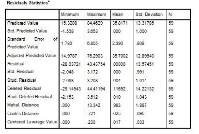
The residuals statistics are values of the regression line, which help to determine whether the errors are near normal distribution. The residuals, also known as the errors, are the differences between the observed values and the predicted value of the dependent variable (Weinberg & Abramowitz 2008). The errors in the time for polishing represent the instant analysis. In the present scenario, the errors are not large, meaning that the model is suitable for the data.
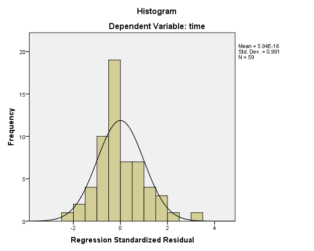
The histogram helps in determining whether the data observes normal distribution. In other words, it checks the normal distribution of the data, which is one of the assumptions that are taken when conducting a regression analysis (IDRE 2015).
In the present scenario, the histogram shows that the data largely observes normal distribution, as the data that lies on the left side of 0 is the same as that on the right side of 0. The normal distribution presented by the histogram shows that the regression model is suitable for this data, as it is one of the assumptions that should be met prior to conducting a linear regression analysis.

The results of the regression analysis can be used to improve the operational efficiency of Nambe Mills and reduce the operations cost. Nambe Mills can lessen the time by making products of smaller sizes, given that the time of polishing increases as the product size increase. This would save time and resources employed in polishing the product and channel the resources into other areas of operations.
The company could assign more personnel to the role of polishing the products that are larger in size, given that they take more time to polish. The company can use the regression equation, Time of polishing = -1.955+ 3.457(diameter), to determine how much time it would require polishing any given item.
Reference List
Carver, R & Nash, J 2012, Doing data analysis with SPSS: Version 18.0, Boston, MA, Brooks/Cole Cengage Learning.
IDRE 2015, Regression with SPSS. Web.
Johnson, R & Kuby, P 2008, Elementary statistics: Enhanced review edition, 10th ed., Thomson Learning, Inc, Boston, MA.
Linear Regression Analysis on SPSS 2015. Web.
Weinberg, SL & Abramowitz, SK 2008, Statistics using SPSS: An integrative approach, 2nd ed., Cambridge University Press, Cambridge, MA.