Introduction
The use of statistical analysis is a valuable strategy for reliable research-based primarily on observable facts. Statistical analysis includes various tools that can be used depending on the ultimate goal of the study. The present paper proposed to identify the reciprocal relationship between the area of a dwelling unit and the price for which it was sold. It was interesting to know if and what effect the floor area had on the final sale price. For the analysis, a set of 1000 data containing information about the region where the dwelling was sold, the listing price, and the square footage. The region of choice was West South Central to make the report more specific.
Representative Data Sample
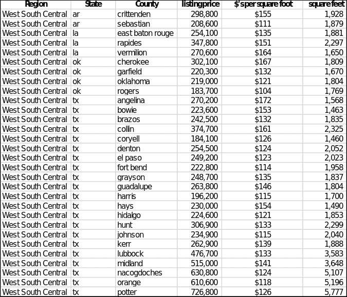
The total number of records for the West South Central region was 100, of which thirty lines were randomly selected, as shown in Figure 1. The average listing price for this sample was $308,483.33 (SD = $140,690.58). The median price value, dividing the data strictly in half, was $254,300.0. Similar scatterplots of descriptive statistics were applied to the floor area variable. The mean square footage of the selected homes was 2319.767 square feet (SD = 1147.928), with the median value calculated as 1880,000.

Data Analysis
A critical aspect of statistical analysis is examining the sample’s representativeness. Although the data were drawn from a national source and were collected by randomly selecting records, there is a risk that the sample unfairly estimates the patterns of the general population. The randomization consisted of removing all the even rows, then fifteen even rows, and then five odd rows, thus maximizing the randomness of the final entries in the sample. Referring to the National Summary Statistics and Graphs Real Estate Data document allows the sample’s representativeness to be evaluated. Specifically, the national average price in the United States was $342,365 (SD = $125,914), while the median value was 318,000. There is a margin of error in the sample statistics compared to the national statistics, but keep in mind that only region-specific data were measured. In terms of housing area, the mean, standard deviation, and median were 2.111, 921, and 1.881, respectively, similar to the data calculated for the sample. Thus, the sample values, although different, were not inconsistent for national statistics, so the sample can be called representative.
Scatterplot
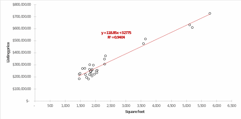
The figure below shows a scatter plot for the relationship of listing price to residential square footage. The x-axis plots the area values (in square feet), and the y-axis represents the listing price (in dollars). In addition, the graph in red illustrates the linear trend graph with the corresponding equation and the value of the coefficient of determination. It is worth clarifying that the R2 determines the fit of the constructed linear model for the data set and determines the share of variance of the point data, which this model covers.

The Pattern
The coefficient of determination for the linear regression was relatively high (R2 =.9404), indicating that this model’s high fit rate covered more than 94 percent of the variance of all data. We can also conclude from the graph that the listing price (y) is generally well described by a linear relationship to the housing area (x), so the area can be used as a predictor. Manipulating the values of this area as an argument of x in the equation in the figure allows us to predict the value of the price. It is reasonable to assume that the model is not strictly accurate, and the calculated coefficient of determination confirms this — there are some outliers: points that are away from the red line. For example, the most apparent outliers include points (2325, $374,700.00) and (3648, $515,000.00). Apparently, for these homes, the prices per square footage significantly differed from the region’s common market price. The reason outliers occur is that linear models are not always valid for real data due to uncertainties and many additional factors, which means there will always be some outliers that lower the coefficient of determination. Finally, linear regression allows predicting the price value based on the specific size of the property. For example, a dwelling of 1,800 square feet, then the predicted price for it would be $246,705.00. The final value of a home around that amount would be predictable and expected by buyers, so it is logical to focus on that value when setting the price.