Introduction
Concern about environmental pollution caused by industrial and domestic activities has grown in recent decades, along with the increasing environmental awareness of the world’s population. A rising number of community groups and organizations are now taking reactive steps to reduce carbon emission levels and shape more sustainable human interactions with the environment (Elçil, 2021). This approach is not surprising given the large body of evidence and projections anticipating the destructive effects of continued climate warming on humanity, animals, and entire ecosystems (Miles-Novelo & Anderson, 2019; Hansen et al., 2020). In the face of increasing concern, it makes sense to turn to numbers as sources of real information to assess relationships and find hidden patterns.
Descriptive vs. Inferential Statistical Analysis
Statistical analysis is a powerful tool for evaluating quantitative data, allowing us to assess relationships between variables, find cause and effect, distinguish between groups, and describe general distribution trends. In this paper, both descriptive and inferential statistical analyses are performed. The former includes measures of central tendency, measures of variability, and the construction of visual representations. Strictly speaking, descriptive statistical analyses refer to recording results in isolation without examining the relationship between variables.
On the contrary, the components of inferential analysis in this paper include conducting t-tests to assess the significance of differences between groups, correlation, and regression tests to measure the strength and direction of the relationship between variables, and assessing the causal effects between them. The measure of significance used for the statistical tests is an alpha significance level of 0.05, which is a classical measure, indicating a low probability of committing a Type I error (Foster et al., 2022). Thus, the statistical analysis carried out in this paper aims at an in-depth mathematical examination of the data describing patterns of global carbon pollution in the atmosphere. The analysis was performed in MS Excel and IBM SPSS, and the results are summarised.
The purpose of this work is to examine environmental data for 62 countries around the world. Indicators of interest include oxygen dioxide emissions per capita, the proportion of a country’s urban population, the proportion of people employed in industry to the total labor force, and GDP per capita. The choice of an approach that calculates carbon dioxide emissions and GDP per capita is appropriate for cross-country comparisons of different regions in terms of population. The main questions to be addressed in this research work are:
- Does a country’s urbanization status affect carbon dioxide emissions?
- Are there significant correlations between the project variables?
- Is there a regression causality for carbon dioxide emissions across countries?
- Can a predictive model be built to estimate potential carbon dioxide emissions?
General Descriptive Patterns
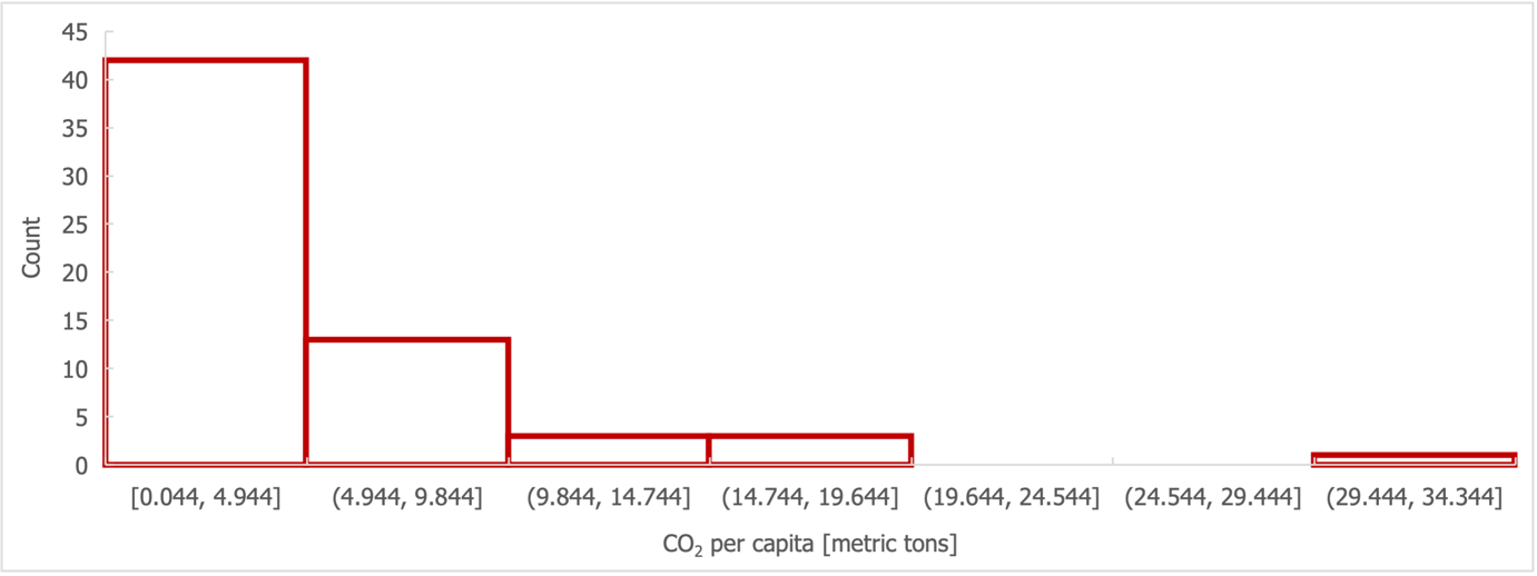
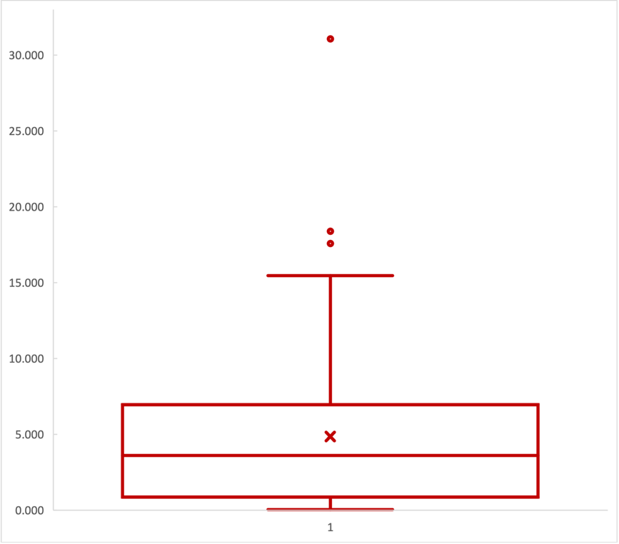
Before conducting an in-depth correlation analysis, general patterns in the distribution of the variables under study must be examined. The sample was represented by 62 countries from almost all continents, including Africa, Asia, Europe, North and South America, and Oceania. The results of the descriptive analysis are summarised in Table 1: as can be seen, for the sample of 62 countries, the mean value of carbon dioxide emissions is 4.85 (SD = 5.52) metric tonnes, with the minimum value being true for Somalia (x = 0.044 metric tonnes) and the maximum for Qatar (x = 31.068 metric tonnes).
The observation that the median of this variable is below the mean by almost 35% may hint at non-normality in the distribution of carbon dioxide emissions. The construction of the histogram (Figure 1) confirms this: the distribution appears right-skewed (Turney, 2023). The boxplot for this variable (Fig. 2) also confirms the presence of the top two outliers in the distribution.
Table 1. Data on mean, median, standard deviation and range for each project variable.
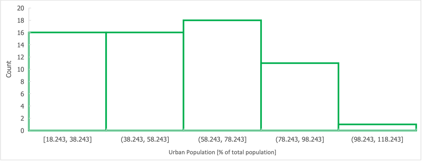
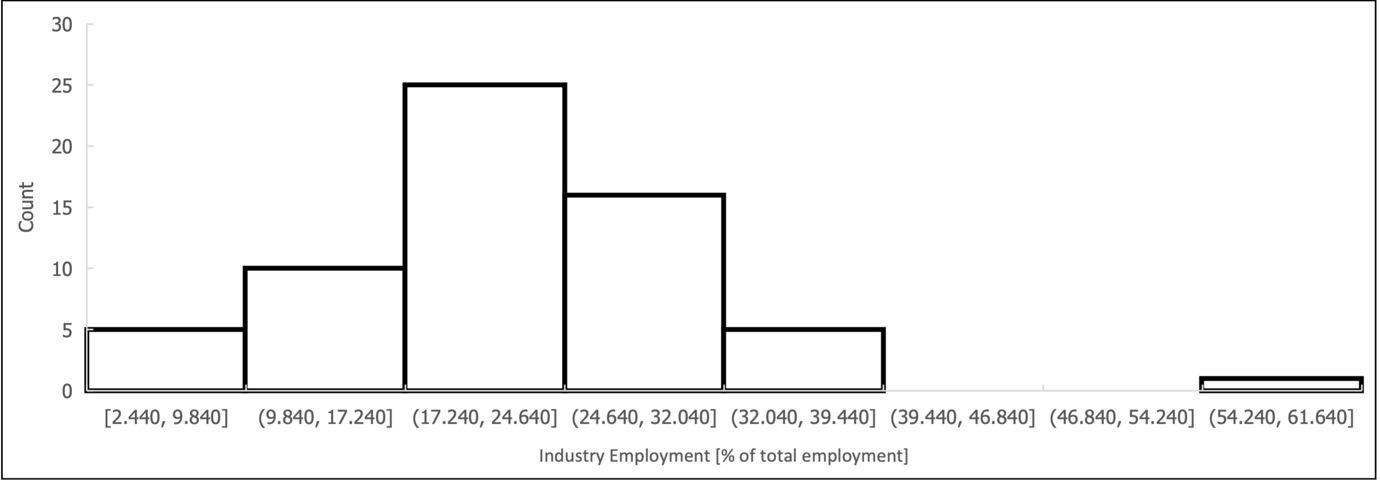
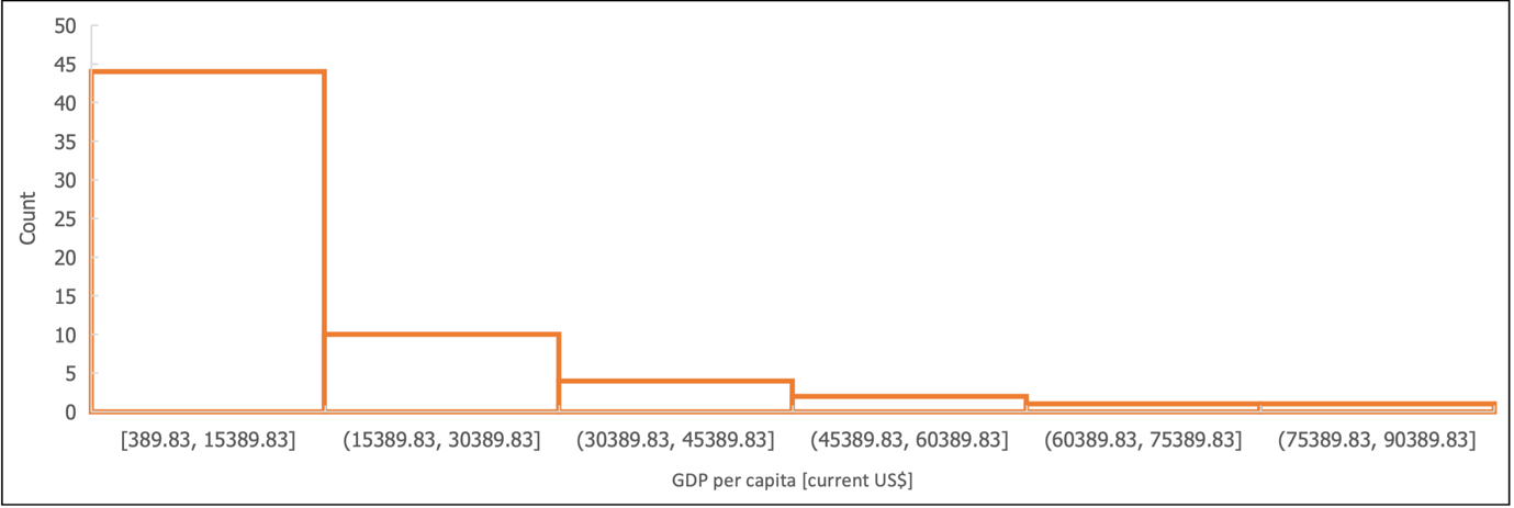
Histograms and boxplots were also constructed for the independent variables to assess symmetric distributions and the presence of outliers. The histograms for the three variables — Urban Population, Industry Employment, and GDP per capita — are shown in Appendix A in Figures 6, 7, and 8. As can be seen from the data, only GDP per capita is characterized by a right-skewed shape, while the other distributions are closer to normality.
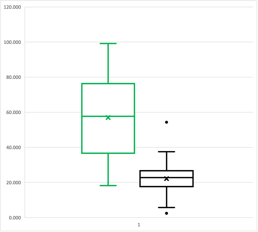
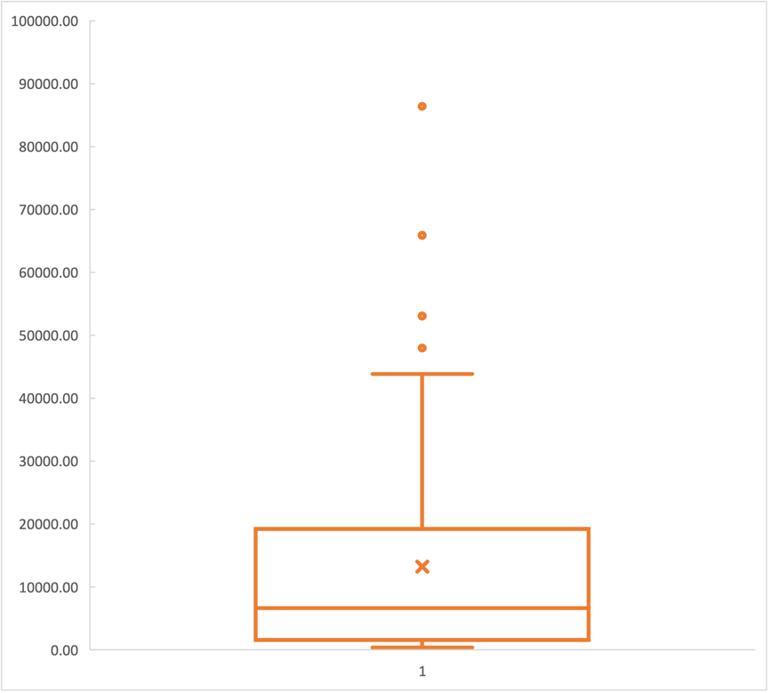
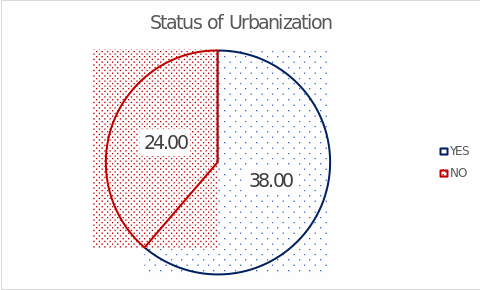
Appendix B shows boxplots for the independent factors: Figure 9 and Figure 10 report that the distributions of Urban Population and GDP per capita had no outliers, in contrast to Industry Employment. Of great interest was the previously unnamed variable determining the urbanization status of a country. Strictly speaking, this categorical variable described whether or not more than half of the country’s population lived in urban areas (UNCTAD, 2021). Figure 3 presents data on the frequency distribution of this status: as can be seen from the data, 38 (61%) countries in the sample were urbanized, and 24 (39%) participating countries were not urbanized.
Since outliers were found in the distribution of the key variable, they were removed because their presence contradicts the assumptions used in further statistical tests. Thus, the United Arab Emirates and Qatar were removed from the sample. Since the GDP per capita variable included the top four outliers (Figure 10), Germany, Netherlands, Qatar, and Switzerland were removed from the sample. Therefore, the final sample thus totaled 57 countries and was used for further analyses.
Impact of Urbanisation Status on Carbon Dioxide Emissions
An important question of the research project was to determine the effect of urbanization status on carbon dioxide emissions. As the independent variable was presented categorically, the dependent variable was a continuous numerical scale, and the number of groups did not exceed two, so a t-test of independent samples was used (Warner, 2020). The null hypothesis of the analysis was that there were no differences in carbon dioxide emissions intensity between the two groups by urbanization status.
In contrast, the alternative hypothesis postulated that there are differences in carbon dioxide emission intensity between the two urbanization status groups. Levene’s test was previously performed to test the assumption of equality of variance distributions (Warner, 2020). The results (Table 2) showed the absence of their equality (F(37.728) = 17.874, p <.001).
The results of the independent samples t-test showed sufficient evidence to reject the null hypothesis and found significant differences between groups (t(37.378) = -6.808, p <.001). This implies that urbanised countries emit significantly more carbon dioxide (M = 6.17, SD = 4.10) than non-urbanised countries (M = 1.09, SD = 1.06). In other words, the urbanization of a country is a predictor of higher carbon dioxide emissions.


Correlation Analysis
As part of the research project, finding whether there were significant correlations between the variables used was interesting. It is worth emphasizing that Pearson correlation cannot be used to formulate cause and effect relationships; it only assesses the direction and strength of the relationship between two variables. The correlation coefficient is from -1 to +1, where +1 corresponds to the strongest positive relationship between variables. As with the t-test, the alpha (.05) level determines the statistical significance of the results (Foster et al., 2022).
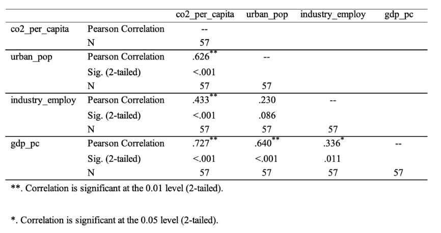
Table 4 presents the results of the correlation analysis performed. As can be seen from the matrix, the level of carbon dioxide emissions is strongly positively correlated with the urban population indicator (r =.626, p <.001). This implies that the higher the urban population in a country, the more emissions are produced per capita. It can be assumed that urban settlements of countries contribute to higher carbon emissions.
In addition, the level of carbon emissions was positively correlated even more strongly with GDP per capita (r =.727, p = <.001). This shows that the wealthier the economy is per capita, the greater the carbon emissions observed. A positive but much weaker correlation relationship (r=.433, p = <.001) was found between the level of carbon dioxide emissions and the proportion of industrial workers employed in the country. From this, the more industry workers are employed, the more emissions are generated. Thus, the level of carbon dioxide emissions was significantly positively correlated with all the quantitative variables of the research project.
These results are not surprising, given the nature of such environmental pollution. Urban populations contribute more than rural populations to emissions, including through personal transport, more intensive public services, and increased creation of daily rubbish (Xiong et al., 2022). The link to the industrialization of society is also logical: more people working in the industries suggests that enterprises play a more important role in a country’s economy: they are more numerous, more widespread, and have higher productive capacity.
In turn, intensive industrial activity directly entails carbon emissions as a by-product of the commercial activity of the enterprise (Xiong et al., 2022). Therefore, the fact that countries with a higher proportion of people employed in industry have higher carbon emissions is not surprising. Higher industrial activity contributes to the enrichment of national economies (Boltanski & Esquerre, 2020). Consequently, GDP per capita increases and people live richer and can afford more goods. For this reason, the ability to generate more carbon emissions is not surprising.
As part of the correlation analysis, observing the potential relationships between the independent variables was also interesting. As shown in Table 4, there is a moderate positive relationship (r=.336, p =.011) between GDP per capita and the proportion of a country’s workers employed in industry. The relationship is much weaker than in the past cases discussed, but still significant.
Hence, as the number of workers involved in the industry generally increases, GDP per capita will also increase. No significant relationship, however, is found between the proportion of the urban population and the proportion of workers involved in the industry (r =.230, p =.086). This indicates no relationship between the variables; thus, it cannot be said that as one variable increases, there is an increase in the other. The latter result is unexpected because, at first glance, the more people living in a city, the more people must labor in the industry to meet the growing needs of the average urban dweller.
Regression Analysis
Regression analysis should also be given attention in a research project. Unlike Pearson correlation, regression analysis tests the effects of independent factors on the dependent variable, which means the results can be used to determine causal relationships (Taylor, 2022). There are both simple and multiple regression analyses, which differ in the number of potential predictors involved. Since the present research project seeks to test the complex influence of independent factors, the choice of both types of regression tests is justified. The significance level of the regression model itself, as well as of each coefficient individually, is tested using a significance threshold of alpha (.05).
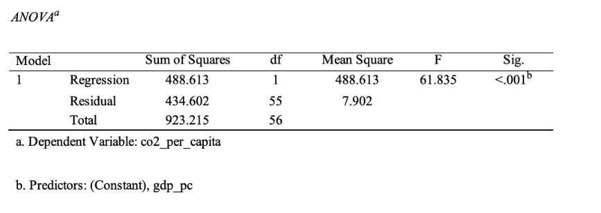
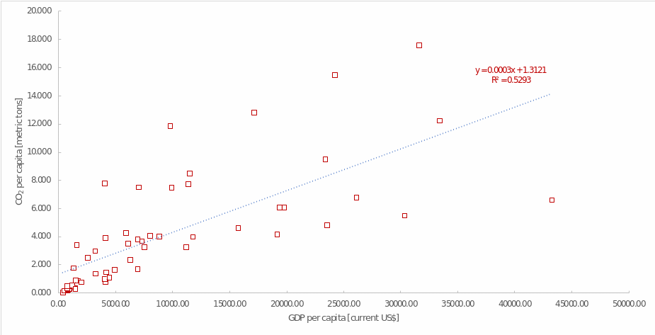
The primary interest was in assessing the effect of GDP per capita on CO2 per capita. Table 5 describes the overall results of this regression model: it is significant and can be used for analysis (F(1, 55) = 61.835, p <.001). Table 6 shows that GDP significantly predicts carbon emissions (B = 0.0003, p = <.001). The plus sign of the coefficient shows that as GDP per capita increases, there is also an increase in CO2 per capita, and for every $1 increase in GDP, the increase in CO2 per capita is 0.0003 metric tonnes. The relationship between the variables is graphically depicted in Figure 4, and it is generally well described by a linear trend.
The coefficient of determination is R2 = 0.529, indicating that this regression model explains up to 53% of the variance in the data set. The final regression equation describing the relationships between GDP per capita and carbon emissions is CO2i = 1.312 + 0.0003∙GDPi. In this equation, the coefficient 1.312 corresponds to the y-intercept, or the value of a country’s carbon emissions at zero GDP, which has no real meaning and is an error in the regression analysis. Otherwise, a simple regression test showed that as GDP per capita increases, and thus the population becomes richer, people tend to have a larger carbon footprint.

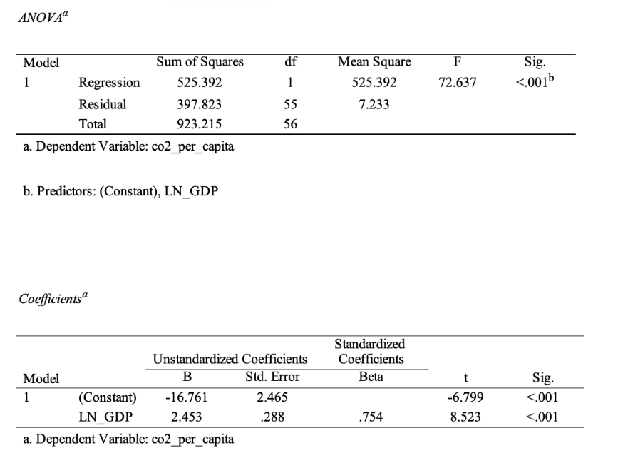
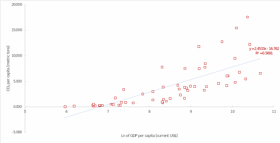
Converting the quantitative variable GDP per capita into the form of a natural logarithm makes sense to linearise the relationship between the variables, stabilise the variance, reduce the negative impact of potentially extreme values and generally improve the quality of the regression model. Table 7 shows that the new regression model is statistically significant, (F(1,55) = 72.637, p <.001), and the results can be analysed. Based on the findings, the natural logarithm of GDP per capita also has statistical significance (B = 2.453, p = <.001). Therefore, if the natural logarithm of GDP per capita increases by one unit, the increase in carbon emissions is 2.453 metric tonnes.
It is not difficult to see that this figure is significantly higher than the one calculated in the previous model. The coefficient of determination in this case also shows an increase and is R2 =.569, or up to 57% of the explained variance. However, due to the use of the logarithmic scale of the independent variable, the y-intercept becomes negative (-16.762) but still makes neither statistical nor economic sense as it describes a non-zero emission at zero GDP. The final regression equation describing the relationships between the natural logarithm of GDP per capita and carbon emissions is CO2i = -16.761 + 2.453∙ln(GDPi). Overall, this model also shows an upward linear trend between the two variables, and the description of this causal relationship is better, as shown by the coefficient of determination.
Multiple regression analysis also makes sense, as it will show the joint influence of two independent factors on the dependent variable. A predictor of employment in the industrial sector has been added to the model, which means that a review of the results will allow us to determine the joint effect of the two independent factors and the effects of this addition on the effects directly from the logarithm of GDP.
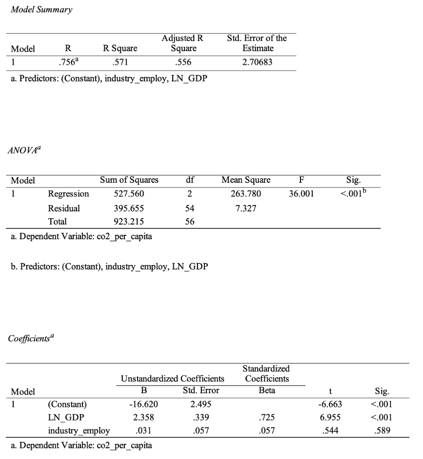
As Table 8 shows, the multiple regression model is statistically significant (F(2,54) = 36.001, p <.001). The coefficient of determination of this model is R2 =.571, which covers a larger percentage of the variance (57.1%) than the two previous regression tests. Notably, GDP retains the statistical significance of the coefficient (B = 2.358, p = <.001). However, the coefficient for the proportion of the population involved in industrialization is not a significant predictor (B = 0.031,p =.589).
In other words, in this model, accounting for the proportion of the population involved in the industry is not statistically significant because, when combined with the natural logarithm of GDP, this predictor is insignificant. Nevertheless, the final regression equation for this model is as follows: CO2i = -16.620 + 2.358∙ln(GDPi) + 0.031∙INDi. The y-intercept remains negative (-16.762) and does not make sense either statistically or economically, as it represents non-zero emissions with a value of zero predictors.
As seen from the several regression tests, the coefficient in front of GDP per capita in logarithmic form varies. Without considering the logarithm, it is 0.0003. With the logarithm, it is 2.453, and in the multiple regression analysis, it is 2.358. The increase in the coefficient between the first and second models is a consequence of the increased linearity of the relationship between the variables and an increase in the overall quality of the regression model. The presence of mixed effects and multicollinearity between predictors can justify the drop in the coefficient in the case of multiple regression models. However, it is important to emphasize that the effect of GDP per capita in a logarithmic form on carbon emissions did not decrease significantly.
The Prediction
The regression model constructed from GDP per capita in logarithmic form and the proportion of individuals employed in the industrial sector can be used for prediction as it showed overall statistical significance. With a GDP per capita of $1,500 and 30% of the population employed in the industrial sector, the carbon emission per capita is calculated as follows:
CO2 = -16.620 + 2.358 ⋅ ln 1500 + 0.031 ⋅ 0.30
CO2 = – 16.620 + 2.358 ⋅ (7.313) + 0.0093
CO2 = – 16.620 + 17.245 + 0.0093
CO2 = 0.634
Hence, the carbon dioxide emission for such a country will be 0.634 metric tonnes. However, the data obtained are estimates and cannot be used to draw precise conclusions.
Conclusion
This research project aimed to investigate the patterns describing carbon dioxide emissions at a global level. The work used a quantitative approach to evaluate the data: descriptive and inferential (t-test, correlations, regressions) statistics were used. The initial sample was 62 countries, but outliers were found when examining boxplots, so five countries were removed. Statistical tests were performed for the 57 remaining countries, illuminating the factors affecting per capita carbon dioxide emissions.
In particular, it was found that an increase in the proportion of the urban population, an increase in the proportion of individuals employed in the industrial sector, and GDP per capita is positively correlated with carbon dioxide emissions per capita. For independent factors, a significant positive correlation was found between GDP per capita and the proportion of industry-employed individuals but not between urban and “industrial” populations.
The results of the statistical analysis also showed that the urbanization status of a country significantly affects the intensity of such emissions. Generally, it was found that the more urbanized a country is, the more carbon emitted. The regression test showed that GDP per capita is a significant predictor of carbon emissions growth in all three models, unlike the proportion of workers employed in industry.
The overall conclusion of this research is that carbon dioxide emissions are influenced by a country’s urbanization, the proportion of people involved in industry, and GDP per capita. Richer, more urbanized, and more industrial countries lead to higher emissions, which is negative for the environment and ecosystems. Consequently, the solution to the problem requires a comprehensive approach, as it cannot be realized through the elimination of the detected factors.
References
Boltanski, L., & Esquerre, A. (2020). Enrichment: A critique of commodities. John Wiley & Sons.
Elçil, Ş. (2021). Environmental awareness in terms of public health: Corporate responsibilities. Akdeniz Üniversitesi İletişim Fakültesi Dergisi, 35, 359-369. Web.
Foster, G. C., Lane, D., Scott, D., Hebl, M., Guerra, R., Osherson, D., & Zimmer, H. (2022). Critical values, p-values, and significance level [PDF document]. Web.
Hansen, B. B., Grøtan, V., Herfindal, I., & Lee, A. M. (2020). The Moran effect revisited: Spatial population synchrony under global warming. Ecography, 43(11), 1591-1602. Web.
Miles-Novelo, A., & Anderson, C. A. (2019). Climate change and psychology: Effects of rapid global warming on violence and aggression. Current Climate Change Reports, 5, 36-46. Web.
Taylor, S. (2022). Regression analysis. CFI. Web.
Turney, S. (2023). Skewness | definition, examples & formula. Scribbr. Web.
UNCTAD. (2021). Total and urban population. Handbook of Statistics. Web.
Warner, R. M. (2020). Applied statistics I: Basic bivariate techniques. Sage.
Xiong, N., Yang, X., Zhou, F., Wang, J., & Yue, D. (2022). Spatial distribution and influencing factors of litter in urban areas based on machine learning – a case study of Beijing. Waste Management, 142, 88-100. Web.
Appendix A
Appendix B
