The trend of gross national income and gross national income per capita
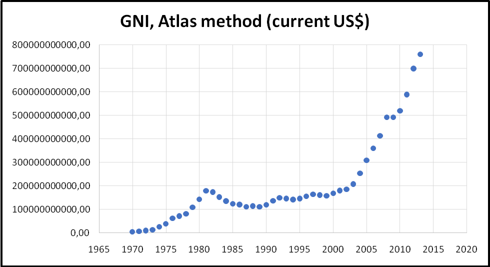
The value of gross national income for the country rose between the years 1970 and 1981. This shows that the income generated by the country rose during the period. The growth rate during this period was 4261.17%. The gross national income declined until the year 1987. The percentage during this period was 36.47%. Thereafter, the value rose again. Further, between the years 1991 and 2003, the country experienced a slow rate of growth.
The total growth rate during this period was 75.18%. Further, from the year 2004, there was a robust growth of gross national income. The total growth rate during the period was 18420.12%. Gross national income grew at different rates during different periods. This trend is consistent with other countries. The graph presented below shows the trend of gross national income for the period between 1970 and 2013.

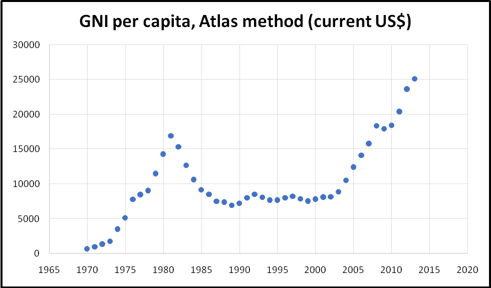
The gross national income per capita also followed a similar trend as gross national income. The graph presented below shows the trend of gross national income per income.

Why gross national income per capita is taken as an effective measure
Gross national income per capita is considered a superior measure of welfare than gross national income. This can be attributed to the fact that it is not underestimated in economies that have low income. Such economies often depend on the informal sector and subsistence activities. Also, this measure adequately reflects the inequalities in income distribution. Also, the gross national income per capita is a useful and readily available pointer that is closely associated with other non-monetary estimates of quality of life. Examples are enrollment rates in schools, life expectancy, and mortality rates among others. Therefore, it does not completely give information on the level of development of a country (Mankiw 2011).
Limitations of gross national income
The first limitation of gross national income is that it makes use of market prices. This ignores the externalities that relate to the environment. However, this limitation can be overcome by the use of accounting prices. The second limitation of using the gross national income is that some expenses that are included in the measure do not necessarily contribute to the well being of the citizens. Therefore, it estimates the social welfare of the citizens. The third limitation is that the gross national income ignores other important aspects of the economy that cannot be quantified in monetary terms (Mankiw 2011). An example is household work. It is often ignored in the calculation of gross national income, yet it contributes immensely to the welfare of the citizens.
Also, the gross national income as a measure of welfare ignores the informal sector of the economy. The informal sector contributes to a greater extent to the welfare of people who live in parts of society that are considered to be poor. Another limitation of the gross national income is that it does not take into account the changes in natural capital that affect the welfare of citizens. For instance, the ecosystem is a vital part of the well-being of the population. Thus, any change in the ecosystem such as water pollution will immensely affect the welfare of the citizens. It is worth mentioning that the valuation of such changes may be quite a problem (Mankiw 2011).
Relationship between life expectancy and income per capita
From the excel file, it can be observed that the correlation coefficient between income per capita and life expectancy at birth is 0.587803. This shows that there is a positive relationship between the two variables. This implies that a higher value of income per capita leads to higher values of life expectancy. This implies that a country that has a high income per capita is likely to have a high life expectancy at birth. It is worth mentioning that correlation does not measure causality between two variables. Correlation is an important element of causality.
In this case, the relationship between life expectancy and income per capita is causal. This is based on the fact that higher-income per capita increases life expectancy. However, this relationship is less noticeable at the highest levels of income per capita. This can be attributed to the fact that at such levels of income lower life expectancy is attributed to old age and lifestyle diseases such as smoking and obesity among others (Mankiw 2011).
Factors that explain the correlation
One factor that explains the relationship between life expectancy and income per capita is the effect of food supply and mortality. With higher income, citizens can afford a constant supply of food and this reduces mortality rates. Also, higher-income implies better access to other necessities in life that increases life expectancy. This leads to higher life expectancy. However, it is worth mentioning that there is a two-way causal relationship between the two variables. For instance, better health increases life expectancy and in turn, increases income (Mankiw 2011).
This is based on the fact that healthy people work longer and harder. Also, a healthy nation positively affects education. For instance, healthy children can stay longer in school and this will positively impact the human capital and in turn, leads to higher levels of income. Also, studies indicate that a healthy nation can save more resources and this leads to the accumulation of physical capital (Gujarati 2014). It also led to the growth of national income. Therefore, the factors that explain the correlation between the two variables can be explained in two ways.
An evaluation of the key drivers of carbon monoxide emissions per capita
This section will focus on establishing if there is a relationship between carbon monoxide emissions per capita as the dependent variable and two independent variables, these are income growth and energy consumption. The relationship between these variables is discussed below.
Scatter plots

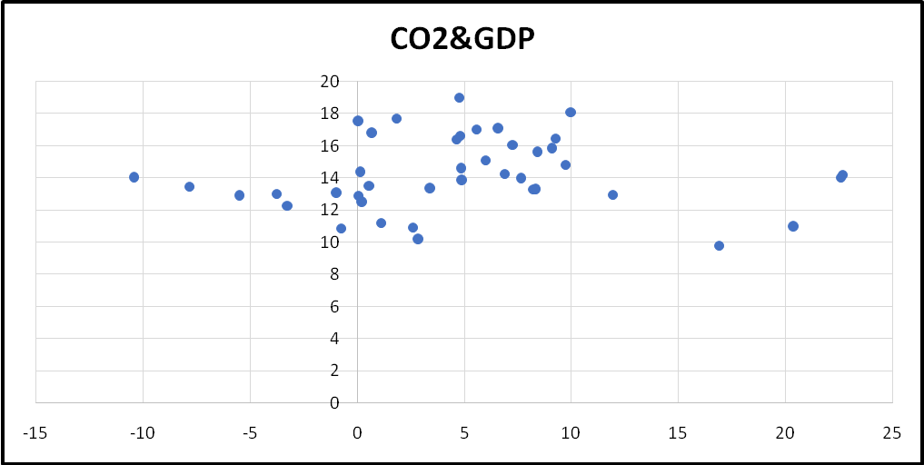
The points in the scatter diagram above do not seem to display a trend. They tend to be in a straight line. This can be an indication that there is a negligible relationship between the two variables.

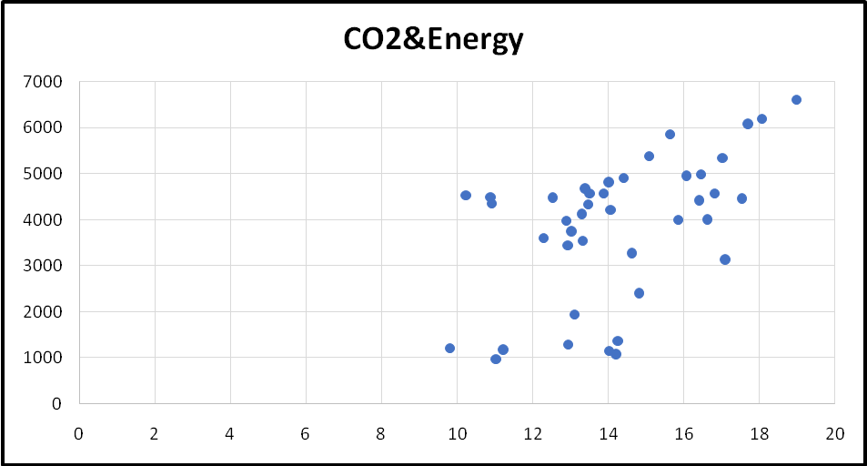
In the scatter plot diagram above, it can be observed that the points are sloping upwards. This shows that there is a positive relationship between carbon dioxide emissions and energy consumption.
Correlations
The correlation coefficient between carbon dioxide emission and income is 0.026454. The value is quite low and it shows that there is a very weak positive linear relationship between the two variables. In the case of energy consumption, the correlation coefficient is 0.521091. This implies that there a positive linear relationship between the two variables. The degree of the relationship is medium (Verbeek 2008).
Regression analysis
Simple regression
The simple regression line will take the form Y = b0 + b1X1
- Y = Carbon dioxide emissions
- X1 = income growth / energy consumption
The theoretical expectations are b0, can take any value and b1 > 0 (positive).
Null hypothesis H0: There is no relationship between carbon dioxide emission and independent variables
Alternative hypothesis H1: There is a relationship between carbon dioxide emission and independent variables.
Results – carbon dioxide emissions and income growth
From the regression results, the equation can be written as Y = 14.2115 + 0.008259X1. The coefficient is positive and it shows that there is a positive relationship between the two variables. Also, the coefficient implies that if a change in income increases by one unit, then carbon dioxide emission will increase by 0.008259 of a unit. The t-calculate (0.165263) is less than the t-critical (1.96). This shows that the change in income is not a statistically significant variable at the 95% confidence level. Also, the value of significance f is 0.869591. The value is greater than the significance level (0.05). This implies that the overall regression line is not significant (Vinod 2008). Finally, the value of the coefficient of determination shows that a change in income only explains 0.07% of variations in carbon emission. The value is low. Therefore, the whole regression line is weak.
Results – carbon dioxide emissions and energy consumption
From the regression results, the equation can be written as Y = 11.27911 + 0.00077X1. The coefficient is positive and it shows that there is a positive relationship between the two variables. Also, the coefficient implies that if energy consumption increases by one unit, then carbon dioxide emission will increase by 0.00077 of a unit. The t-calculate (3.8128) is greater than the t-critical (1.96). This shows that energy consumption is a statistically significant variable at the 95% confidence level. Also, the value of significance f is 0.000477. The value is less than alpha (0.05). This implies that the overall regression line is significant (Greene 2008). Finally, the value of the coefficient of determination shows that energy consumption explains only 27.15% of variations in carbon emission. The value is low. Therefore, energy consumption is a statistically significant variable.
Multiple regression analysis
The multiple regression line will take the form Y = b0 + b1X1 + b2X2.
- Y = Carbon dioxide emissions.
- X1 = income growth.
- X2 = energy consumption.
Results
The multiple regression equation can be written as Y = 10.067 + 0.0951X1 + 0.000963X2. The coefficients are positive and it shows that there is a positive relationship between the dependent variable and the independent variables. Also, the coefficient implies that if a change in income and energy consumption increases by one unit, then carbon dioxide emission will increase by 0.0951 and 0.000963X2 of a unit respectively. The values of t-calculate are 2.1025 and 4.4935 for income growth and energy consumptions respectively. The values are greater than the t-critical (1.96).
This shows that the two variables are statistically significant at the 95% confidence level. Also, the value of significance f is 0.0003. The value is less than alpha (0.05). This implies that the overall regression line is significant. Finally, the value of the coefficient of determination shows that two variables explain only 34.74% of variations in carbon emission. The value is low. It can be observed that additional variables improve the regression model (Baltagi 2014). The analysis above shows that there is no causal relationship between carbon emission and change in income. Income growth does not cause carbon emissions to rise.
References
Baltagi, G, (2014). The oxford handbook of panel data. Web.
Greene, W, (2008). Econometric analysis. Web.
Gujarati, D, (2014). Econometrics by example. Web.
Mankiw, G, (2011). Principles of economics. Web.
Verbeek, M, (2008). A guide to modern econometrics. Web.
Vinod, D, (2008). Hands on intermediate econometrics using r: Templates for extending dozens of practical examples. Web.