- Introduction
- The histogram of day 1 variable
- The normal probability plot of hygiene day 1 of download festival
- Exploring day 3 of download festival
- The above table 1 shows the value of descriptive statistics of the variables
- The description of numeracy and computer literacy
- The test of homogeneity
- Assumption violation
- References
Introduction
Why do we do a normal test?
A normal test is usually done to ensure that the data is normally distributed since the test statistics used follows a normal distribution.
Activity One
Data exploring
In this study, we are interested in exploring the festival data if there are normally distributed. In this study, we are going to explore the festival data using the histogram and normal probability plot of the festival data (Ball, 2001). The festival data consist of three variables day 1, day 2, and day 3. We will investigate if all the three variables follow a normal distribution. We will also have the frequency table of the tree variables.
The histogram of day 1 variable
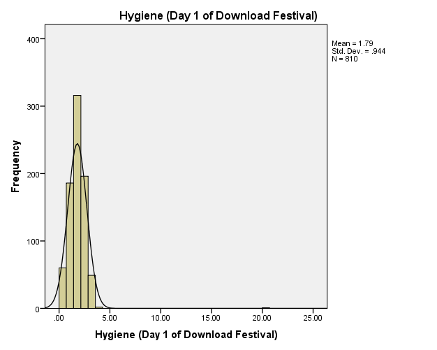
From the day one histogram, we can observe that the value of the mean is equal to 1.79, the standard deviation is equal to 0.944 and the value of observation is 810. From the histogram, we can observe that the festival data of day one is normally distributed about the mean of the data. We can also observe that the festival data is symmetrical about the mean of the day 1 of download festival. This means that the day 1 of download festival can be used to conduct analysis where the normal assumptions have been made.
The normal probability plot of hygiene day 1 of download festival
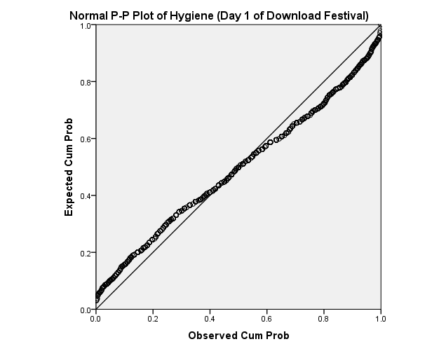
The trended hygiene data of day 1 of download festival show that the data is normally distributed. This is indicated clearly because the residual p-p plot of the day 1 of download festival data of hygiene are close to the line implying that the errors and the festival data re normally distributed.
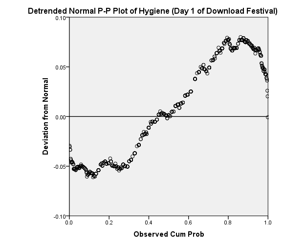
The normal probability plot of the hygiene festival data is not normally distributed when the data has not been trended. The plots of the error are very far from the line implying that data is not normally distributed.
The exploring of hygiene day 2 of download festival
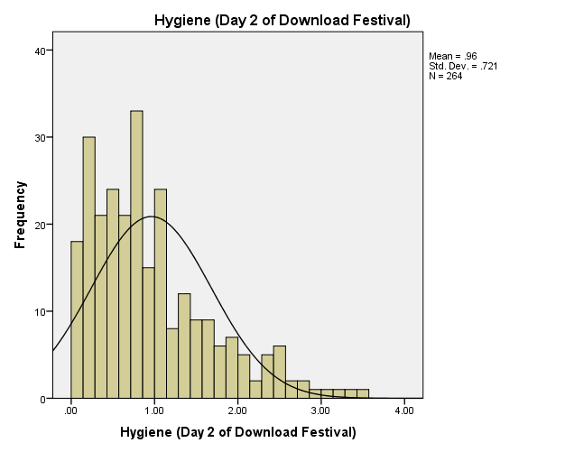
From the day one histogram, we can observe that the value of the mean is equal to 0.96, the standard deviation is equal to 0.721 and the value of observation is 264. From the histogram, we can observe that the festival data of day one is not normally distributed about the mean of the data. We can also observe that the festival data is not symmetrical about the mean of the day 2 of download festival. This means that the day 2 of download festival can be used to conduct analysis where the normal assumptions have been made (Kutner, Nachtsheim, Neter & Li, 2005).
The normal probability plot of hygiene day 2 of download festival
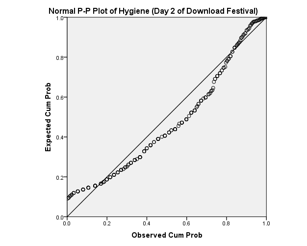
The trended hygiene data of day 2 of download festival show that the data is normally distributed. This is indicated clearly because the residual p-p plot of the day 2 of download festival data of hygiene are close to the line implying that the errors and the festival data re normally distributed.
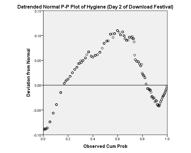
The normal probability plot of the hygiene festival data is not normally distributed when the data has not been trended. The plots of the error are very far from the line implying the data is not normally distributed.
Exploring day 3 of download festival
The histogram of the hygiene day 3 of download festival
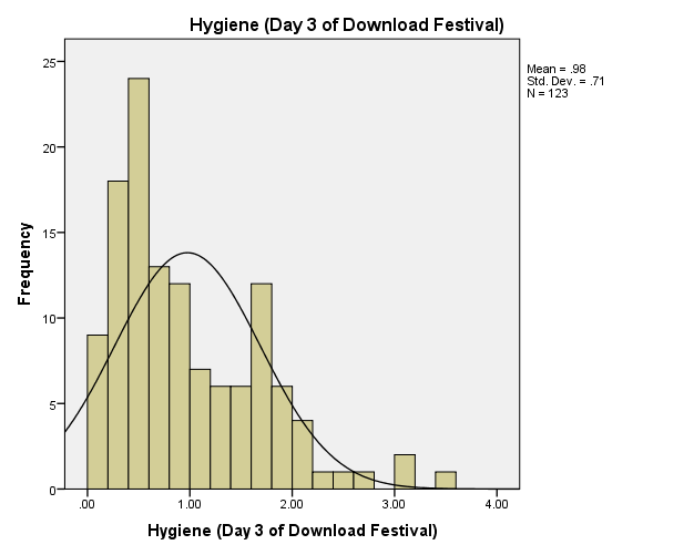
From the day 3 of download festival histogram, we can observe that the value of the mean is equal to 0.98, the standard deviation is equal to 0.71 and the value of observation is 123. From the histogram, we can observe that the festival data of day 3 is not normally distributed about the mean of the data. We can also observe that the festival data is not symmetrical about the mean of the day 3 of download festival. This means that the day 3 of download festival can be used to conduct analysis where the normal assumptions have been made. The hygiene data of day 3 download festival has two outliers and for the download festival data of day 3 to be used in any analysis that need normal assumption we need the outliers to be removed and transformed to normal.
The normal probability plot of the hygiene day 3 of download festival
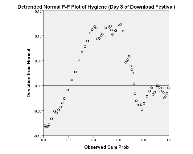
The normal probability plot of the hygiene festival data is not normally distributed when the data has not been trended. The plots of the error are very far from the line implying that data is not normally distributed.
The descriptive statistics of the download festival
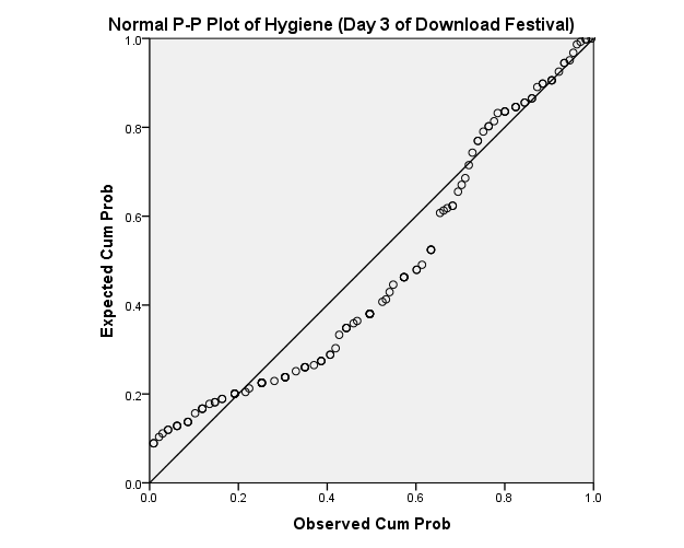
The trended hygiene data of day 3 of download festival show that the data is normally distributed. This is indicated clearly because the residual p-p plot of the day 3 of download festival data of hygiene are close to the line implying that the errors and the festival data re normally distributed.
The above table 1 shows the value of descriptive statistics of the variables
From the descriptive statistics, the variable day one had no missing value. The mean of hygiene day one of download festival is 1.7934, the median is 1.79, the variance is 0.892, the kurtosis statistic is 170.45, and the skewness statistic is 8.865. The variable hygiene day two of download festival had 546 missing values, the mean of 0.9609, the median is 0.79, the variance is equal to 0.52, the value of skewness statistic is 1.095 and the value of kurtosis is 0.822. The variable hygiene day three of download festival has 687 missing value, the mean of 0.9765, median is 0.76, the variance of 0.504, the skewness statistic of 1.0033, and the kurtosis statistic of 0.732.
From the skewness value we can say that the day I of download festival is skewed to the right of the mean, the standard error of the skewness statistic is 0.086. The skewness value is 1.095.
The description of numeracy and computer literacy
From the descriptive statistic of table 2, the total sample was equal to 50, the mean value is 4.12, the median is 4, the standard deviation is equal to 2.067, the skewness is 0.512 and the kurtosis statistic is -0.484. From the skewness statistic, we observe that the value of the skewness is negative hence the data is skewed to the left of the mean of the data.
The descriptive statistic of the numeracy and the computer literacy at university of Sussex University
From the descriptive statistic, the total sample was equal to 50, the mean value is 5.58, the median is 5, the standard deviation is equal to 3.071, the skewness is 0.793, and the kurtosis statistic is 0.26. From the skewness statistic, we observe that the value of the skew ness is positive hence the data is skewed to the right of the mean of the data.
The histogram of the numeracy
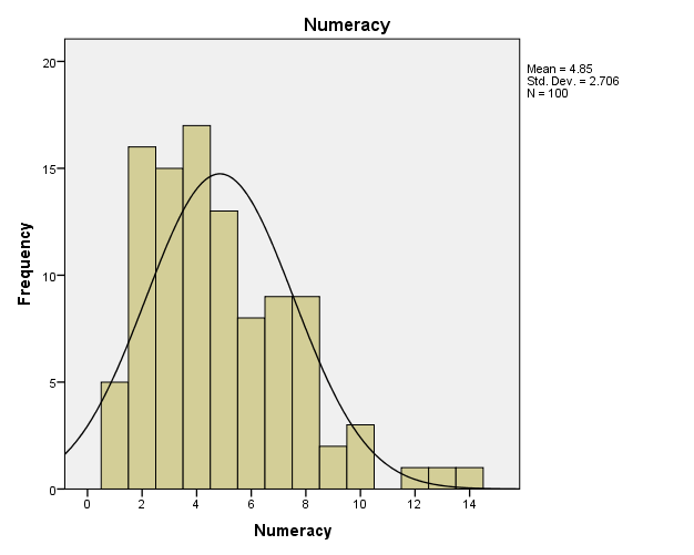
From the histogram the numeracy of the university dunce town is skewed to the right.
The numeracy data is not symmetrical about the mean. The numeracy contains the outliers.
The histogram of computer literacy
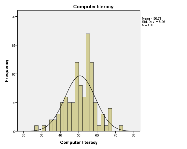
From the histogram of the computer literacy, we can see that the data on computer literacy is normally distributed about the mean. The data on computer literacy has three outliers.
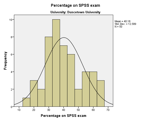
The test of homogeneity
From the test of homogeneity of variance, the levene statistic of computer literacy is 0.064 with a significant value of 0.801 which is greater than 0.05. This means that we fail to reject the hypothesis that the variances are homogeneous. We therefore conclude that the variance of computer literacy is homogeneous. The value of the levene statistic is equal to 1.731 with a significant value of 0.191. This means that we fail to reject the hypothesis that the variance is homogeneous. We therefore conclude that the variance is homogeneous.
We can able observe from the test of homogeneity of variance table that the values of significant are all greater than the 0.05. This mean that we fail to reject the hypothesis that the variance is homogeneous and we conclude that the variance of the computer literacy and the percentages of lectures attended have their variance homogeneous based on both median and trimmed mean.
Assumption violation
When assumption of homogeneity of variance is violated, the data fail to obey the normality assumptions. This lead to contradicting conclusions hence there is over dispersion of the parameters.
References
Ball, K. S. (2001). The Use of Human Resource Information Systems: a Survey. Personnel Review, 30(6), 667- 693.
Kutner, M., Nachtsheim, C., Neter, J., & Li, W. (2005).Applied Linear Statistical Models (5th ed.). New York: McGraw-Hill/Irwin.