Executive summary
The paper made use of the Two-Fund Theorem to find a solution to the asset and capital allocation problem. The monthly stock prices for Procter & Gamble and Royal Bank of Canada are used for the analysis. The discussion on the asset allocation problem focuses on locating the minimum variance portfolio on the efficient frontier of the two assets. At the point of the minimum variance portfolio, the weight of the two securities is 83.41% and 16.59% for Procter & Gamble and Royal Bank of Canada respectively. The effect of altering correlation on portfolio variance is also discussed. It is established that it is possible to create a perfect hedge when the two securities are perfectly correlated. Also, it is established that diversification reduces the portfolio variance thus leading to a minimization of unsystematic risk. In the second part, the capital allocation problem is solved using the Single Index and Treynor-Black model. The weight allocated to an active portfolio is 54.12%, while the weight allocated to a passive portfolio is 46.88%. Finally, a review of data for the two companies at a later date shows that the efficient market hypothesis holds.
Introduction
The paper seeks to discuss the two parts of the Two-Fund Separation theorem. The premise of this theorem is the modern portfolio theory. According to the Two-Fund Separation theorem, an investment problem is separated into two steps. The first step entails allocating resources between two or several risky assets. It focuses on analyzing the efficient frontier of the assets in the portfolio to solve the asset allocation problem. The second step seeks to find an optimal solution between risk-free and risk assets. In this case, the Treynor-Black framework will be used to find an optimal solution. These two parts are discussed in the subsequent sections.
Analysis of security
The securities that will be analyzed are the stocks of Proctor & Gamble Co. and Royal Bank of Canada. Both companies are publicly traded entities that are listed on the New York Stock Exchange market with ticker symbols PG and RY respectively. However, the stock of Royal Bank of Canada is listed on the other two stock exchange markets. Further, Proctor & Gamble Co. Deals with the production and sale of a variety of consumer goods while Royal Bank of Canada offers financial services. The table presented below shows a summary of financial data for the two companies.
(Source of data – Yahoo, Inc. 2009a; Yahoo, Inc. 2009b)
The data show that Proctor & Gamble Co. has a high earnings capacity while Royal Bank of Canada has a large asset base. For subsequent analysis, the share prices of the companies will be collected. These prices will be used to calculate the monthly return for each stock. The data of stock of the two companies, the S&P 500 index and 60-day Treasury Bill is presented in appendix 1 (Yahoo, Inc. 2009c). The table presented below shows a summary of the results for portfolio analysis.
The results show that Proctor & Gamble Co. has a higher expected return and lower standard deviation than Royal Bank of Canada. Further, there is a weak positive correlation between the monthly return of the two stocks.
Asset allocation problem (AAP)
Most investors often face the asset allocation problem. This is a problem that arises when an investor seeks to allocate resources between several risky assets. Therefore, an investor needs to find an optimal portfolio of risky securities. In this case, there are no risk free assets (Elton & Brown 2007). The calculations for this section are presented in appendix 2 below.
Optimization and the efficient frontier
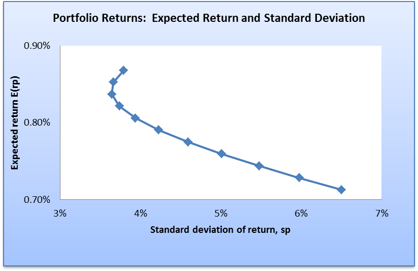
In order to solve the asset allocation problem, it is important to estimate the expected return and standard deviation of a portfolio. The estimated value of expected portfolio return is 0.79%, while the portfolio variance is 0.18%. The portfolio standard deviation is 4.23%. The calculations are based on the assumption that the two stocks have equal weights. The next step is to come up with an array of possible combinations of expected returns and standard deviations of the two stocks. The combinations will be plotted on a graph. The resulting graph is a frontier which shows all possible combinations of risk and return of the portfolio (Elton & Brown 2007).
Central tendency portfolio
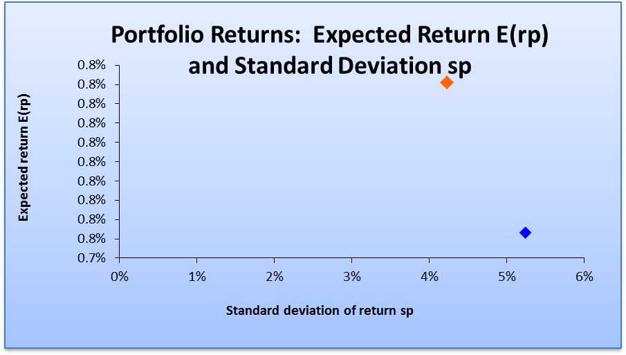
This represents a portfolio that is based on the measures of central tendency. The position of this portfolio is presented in the graph below.
Minimum variance portfolio
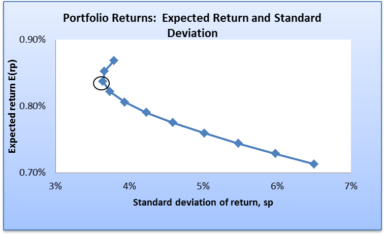
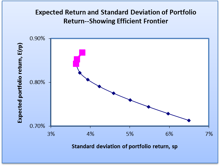
This represents a portfolio that is associated with a minimum of risk. That is, it has the least value of variance. This portfolio is also associated with minimum return. This argument is based on the fact that there is a direct relationship between risk and return. Thus, risky assets attract high returns. In the case of the two companies, the minimum variance portfolio is attained at the point where the weight of Proctor & Gamble stock is 83.41%, while that of Royal Bank Canada is 16.58%. The portfolio variance is 3.64%, while the expected return is 0.84%. The graph presented below shows the minimum variance portfolio.
Maximum variance portfolio
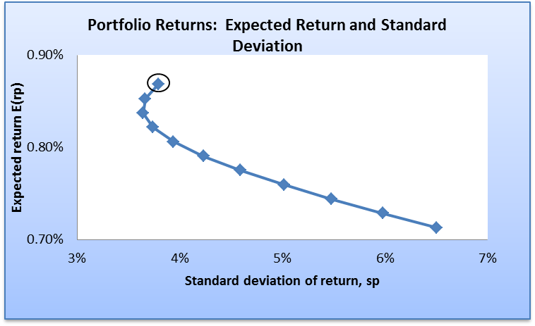
This portfolio generates the maximum return to an investor. Therefore, it is associated with high level of risk. In the case of the two companies, the maximum variance portfolio is attained at the point where the weight of Proctor & Gamble stock is 100%, while that of Royal Bank Canada is 0%. The portfolio variance is 3.79%, while the expected return is 0.87%. The graph presented below shows the maximum variance portfolio.
Efficient frontier
This represents the section of the frontier curve that lie between the minimum and maximum variance portfolio. The points on the efficient frontier offer a higher amount of return at a given level of risk or they have a low level of risk at a specific level of return. The efficient frontier of the two companies is highlighted in pink in the diagram below.
Correlation and portfolio variance
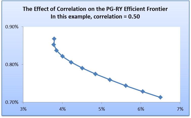
There are a number of approaches that can be used to estimate the variance of a portfolio. One approach is by using the correlation coefficient. Therefore, changing the value of correlation coefficient affects the variance of a portfolio. This creates the need for evaluating the impact of changing the values of correlation coefficient on the risk level of a portfolio. The analysis will be carried out fewer than three scenarios. In the first scenario, it will be assumed that the correlation between the two stocks is 0.5. The resulting frontier curve is presented below.
In the second case, it will be assumed that the correlation coefficient is 1. The frontier curve will change to the shape presented in the diagram below.
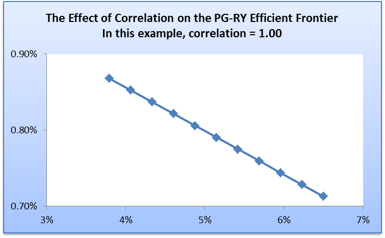
The graph is a straight line that is downward sloping. It is similar to a scenario where a portfolio contains ne risk free asset and one risky asset. The correlation coefficient of 1 indicates that the two assets are perfectly correlated. Thus, an investor can come up with a perfect hedge that comprises of two assets. The final instance is when the correlation coefficient is -1. The shape of the frontier will change as presented below.
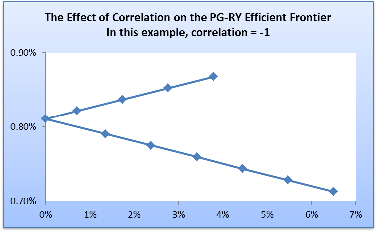
In this case, there is a perfect negative correlation between the two assets. Thus, it is possible to form an artificial risk free asset. However, the shape gives indication that one security in the portfolio dominates another one.
Systematic risk, Nonsystematic risk and diversification
When finding a solution to the asset allocation problem, it is important to evaluate the concept of diversification. This can be explained by the fact that some risks that are associated with investing in some securities can be minimized. Risks can be can be classified as either systematic or nonsystematic risks. Systematic risks are inherent in a market. Therefore, they cannot be eliminated by investing in a variety of stocks. This type of risk is often measured using the beta. The return on stock for Proctor & Gamble Co. has a beta value of 0.0163. This implies that the stock has less movements a compared to market volatility. On the other hand, Royal Bank of Canada has a beta value of -0.0744. Thus, share prices move in opposite direction as compared to the market. Thus, in the case of systematic risk, the stocks of various companies will tend to move in a similar direction. Unsystematic risk is the uncertainties that relate to a single entity. This type of risk can be reduced by having a portfolio that has several assets.
The proponents of diversification argue hat the risk – return tradeoff improves when an investor invests in several assets that are not perfectly correlated. From a mathematical point of view, as the number of assets in a portfolio increases, then the covariance between the assets moves close to zero. Thus, the variance of the portfolio also reduces. This occurs only when the covariance of the portfolio is negative.
Capital allocation problem (CAP)
Capital allocation is an important aspect of investment. This is based on the fact that resources are scarce. Therefore, an investor needs to find a suitable approach of coming up with an optimal weight of allocating capital among the securities. There are several approaches that can be used to arrive at an optimal way of allocating capital. The first approach is by picking the point of tangency of the capital asset line and utility function. This point will yield optimal weights. The second method is by using the single model and Treynor-Black framework. The capital allocation problem in this case will be solved using a combination of these two models. The capital allocation problem concentrates on the second part of the Two-Fund Separation theorem. Therefore, it will seek to find an optimal solution when allocated resources between a risk free and a risky asset. The calculations are presented in appendix 3 below.
Single index model
This model shows the relationship between the returns on each security to the returns of the market index. In this case, the market index is the S&P 500 index. It measures the risks and return of a security. This model splits the total risk of an asset into market risk (measured by beta) and unique risk (measured by alpha). The values of alpha and beta for the single risk model will be solved using regression analysis. The results of regression for the two stocks are summarized in the table below.
The results in the table above show that Proctor & Gamble Co. has a higher value of unique risk than Royal Bank of Canada. Also, Proctor & Gamble Co. is less sensitive to market movement (as indicated by the value of the beta). On the other hand, the stock of Royal Bank of Canada moves in the opposite direction of the market. This is explained by the negative value of beta. The results of the single index model are a significant input to the Treynor-Black model.
Treynor-Black framework
This framework provides an efficient approach of implementing an active investment strategy. In this model the optimal portfolios are built using the actual forecasts of abnormal returns and the coefficients of beta. This framework works by identifying active portfolio that can be blended with passive portfolio to find the optimal risky portfolio. Further, weights are assigned to the securities proportionately. Thus, securities that have low levels of unsystematic risks are allocated more weight. The framework is built on one major key assumption. That is, the market is assumed to be efficient. This might not be always the case because degree of efficiency of the market depends on a number of factors. The process of using this model goes through several distinctive steps. These steps are discussed below.
Step 1
The first step is to ensure that there are values of beta and alpha of stocks. These values are already estimated using the single index model above. The values of beta and alpha will aid in the calculation of the factor models as presented below.
Step 2
This step entails calculating the weight of stock in the active portfolio. There exist a direct proportionality between the weights and the ratio of alpha and unsystematic risks. This ratio is commonly known as the appraisal ratio. It captures the value that a security adds to the portfolio. The direct proportionality indicates that securities that have higher values of alpha (Proctor & Gamble Inc.) are allocated more weights than those with lower values of alpha (Royal Bank of Canada) as presented in the table below.
The estimated weight for Proctor & Gamble is 75%, while that of Royal Bank of Canada is 25%.
Step 3
This will focus on estimating the weighted averages of beta, alpha, and idiosyncratic risk of the active portfolio. The results are presented in the table below.
Step 4
At this point the weight of the active portfolio will be calculated using the formula presented below.

The estimated weight of the active portfolio is 118.85%.
Step 5
This step is quite important because it focuses on correcting the adjusted beta of the active portfolio. This correction is quite important because it ensures that there is no significant deviation of the portfolio beta from the overall beta. It also ensures that the overall portfolio does not become too risky. The outcome of this step is a corrected value of beta, which is 54.12%. This will represent the weight of the active portfolio (Bodie, Kane & Markus 2012).
Step 6
The final step entails calculating the weight of passive portfolio. The sum of weights of active and passive portfolios should be 1. Therefore, the weight of the passive portfolio is 45.88% (100% – 54.12%). Therefore, the results indicate the ratio of how the resources will be allocated. This represents the solution to the capital allocation problem.
Efficient market hypothesis
The concept of efficient market hypothesis was developed in 1960 by Eugene Fama. The idea has widely been used across the market. The underlying concept of the hypothesis is that all available information in the market is replicated in the prevailing market prices (Baltagi 2011). Thus, if information about a security is available, then it is quickly replicated in the market price of the security. Therefore, there is no room for using such kind of information to make undue gain. The degree of efficient market hypothesis differs depending on the type of the information and the rate at which the information is assimilated in the market price of the security. The underlying concept of efficient market hypothesis is consistent with the random walk hypothesis.
Evaluation of portfolio at a later time period
The prices of stocks of the two companies will be collected for the period between between the period 03/03/2013 and 06/03/2014. Once the closing prices of stock for the two time periods are collected, then the monthly returns of stock will be calculated. The value of returns will be arrived at by calculating the monthly percentage change of stock prices. Further, the average of the monthly returns of the two stocks will be computed. A portfolio will be created using the data of monthly rate of return of the two stocks using the optimal weights calculated above. The portfolio mean for the two time periods will be calculated and compared. The calculations are presented in appendix 4 below. The table presented below shows a summary of the results.
The information in the table above shows that there is a difference in expected return between the two time periods. The expected returns of the portfolio for the period between 03/03/2013 and 06/03/2014 are higher than those of the period between 01/03/2010 and 01/03/2013. Thus, it can be noted that there is a clear indication that the expected portfolio return of the two time periods are different. The portfolio performed better at a later time period. This can be an indication that the past trends of stock prices did not have an impact on the future prices. Thus, there is no replication of past trend in the future (Elton & Brown 2007).
Conclusion
In summary, the discussion on the asset allocation problem focuses on locating the minimum variance portfolio on the efficient frontier of the two assets. At the minimum variance portfolio point, the weight of the two securities is 83.41% and 16.59% for Procter & Gamble and Royal Bank of Canada respectively. In the second part, the capital allocation problem is solved using the Single Index Model and Treynor-Black model. The weight allocated to active portfolio is 54.12%, while the weight allocated to passive portfolio is 46.88%. Finally, a review of data for the two companies at a later date shows that the efficient market hypothesis holds for the two securities.
Reference list
Baltagi, G 2011, Econometrics, Springer, New York.
Bodie, Z, Kane, A & Markus, A 2012, Investments, McGraw Hill Publishing Company, USA.
Elton, G & Brown, G 2007, Modern portfolio theory and investment analysis, John Wiley & Sons Ltd, USA.
Yahoo, Inc. 2009a, The proctor & gamble company (PG).
Yahoo, Inc. 2009b, Royal bank of Canada (RY.
Yahoo, Inc. 2009c, S&P 500 (˄GSPC).
Appendices
Appendix 1 – Data
Proctor & Gamble Royal Bank of Canada Portfolio
Appendix 2
PORTFOLIO STATISTICS for a Proctor & Gamble-Royal Bank of Canada Portfolio
Portfolio return and risk
PORTFOLIO STATISTICS for a Proctor & Gamble-Royal Bank of Canada Portfolio
Portfolio return and risk
Possible combinations
Maximum variance portfolio
Minimum portfolio variance
Efficient Frontier
Effect of correlation coefficient on the portfolio
Correlation coefficient of 0.5
Possible combinations
Correlation coefficient -1
Possible combinations
Correlation coefficient 1
Possible combinations
Appendix 3
Single Index Model
Regression results
Proctor & Gamble
Royal Bank of Canada
Treynor-Black Framework
Results
Results estimation factor models
Determine stocks weights active portfolio
Determine alpha, beta, and idiosyncratic risk of the active portfolio
Determine weight active portfolio – 118.85%
Perform correction to adjust beta active portfolio – 54.12%
Determine weight passive portfolio – 45.88%
Appendix 4
Analysis at a later time period
Data
Portfolio data
CALCULATING PORTFOLIO RETURNS AND THEIR STATISTICS
Direct calculation of portfolio mean and variance