Executive summary
The discussion in the paper focuses on the Two-Fund Separation theorem. It is an expansion of the modern portfolio theorem. The data of adjusted closing prices for Proctor & Gamble Co. and Royal Bank of Canada is used in the analysis. An analysis of the securities shows that the two companies operate in different industries and they have different sizes. The discussion also reveals that the asset allocation problem focuses on the allocation of resources between two risky assets. Further, diversification helps in minimizing non-systematic risks when investing in risky assets. The capital allocation problem focuses on the allocation of resources between risk-free and risky assets. The optimal point of allocation is estimated using the Treynor-Black model.
Introduction
The paper seeks to use the Two-Fund Separation theorem to solve the asset and capital allocation problem. This theorem is an expansion of the modern portfolio theory that was developed by Harry Markowitz in the 1960s (Elton & Brown 2007). The portfolio theory outlines that investors need to control the risk of their portfolio by allocating resources between risky and risk-free assets. Thus, risk cannot be controlled by rearranging resources among risky assets. The theory also maintains that a portfolio should be well-diversified. Therefore, a portfolio of risky assets should contain several assets. The first part of the Two-Fund Separation theorem will be used to solve the asset allocation problem. It will focus on allocating resources between two or more risky assets. This section will focus on analyzing efficient frontier. The second part of the theorem will solve the capital allocation problem. In this case, the Treynor-Black model will be used to allocate resources between risk-free and risky assets.
Security analysis
The paper focuses on analyzing the stock for Proctor & Gamble Co. and Royal Bank of Canada. Proctor & Gamble Co. is a public company that is based in the United States. It trades on the New York Stock Exchange with the ticker symbol PG. Besides, it is a component of the S&P 500 index and the Dow Jones Industrial average. The company deals with the production of assorted consumer goods. From a financial point of view, the revenue of the company grew from $78,938 million to $84,167 million in 2013 while the net income dropped from $12,736 million in 2010 to $10,756 million in 2012. The value rose to $11,312 million in 2013. The total assets of the company fluctuated during the period. The balance in 2013 was $139,263 million. On the other hand, Royal Bank of Canada is also a public company that is based in Canada. The company trades on 3 stock exchange markets one of them is the New York Stock Exchange. The company’s ticker symbol is RY. Further, it operates in the financial services industry. The company prepares the financial statements using Canadian dollars. The revenue grew from CAD28,330 million in 2010 to CAD30,867 million in 2013. Further, the net income dropped from CAD5,223 million in 2010 to CAD4,852 million in 2011. The value later grew from CAD7,442 million in 2012 to CAD8,331 million in 2013. The total assets of the Bank amounted to CAD860,819million in 2013 (Yahoo Inc. 2009a; Yahoo Inc. 2009b; Yahoo Inc. 2009c).
Thus, a comparison of books of account for the two companies shows that Proctor & Gamble Co. has higher revenue and net income than Royal Bank of Canada. However, Royal Bank of Canada has a larger asset base than Proctor & Gamble Co. The data of closing share prices and rate of return are presented in Appendix 1. The average rate of return for PG is 0.87%, while for RY is 0.71. Further, PG has a variance of 0.0014 and a standard deviation of 3.79%, while RY has a variance of 0.0042 and a standard deviation of 6.5%. Thus, it can be noted that PG has a higher rate of return and lower risk (standard deviation and variance) than RY. This can partly be attributed to the fact that Royal Bank of Canada operates in an extremely risky industry that offers low returns. The covariance between the two securities is 0.0007 while the correlation coefficient is 0.3029. This shows that there is a weak positive association between the two securities. The graph presented below shows the relationship between the returns of the two securities.
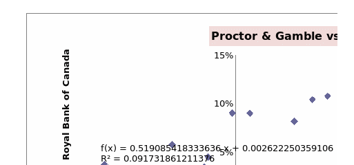
Apart from the data of the two companies, the closing prices for S&P 500 index and interest rate for the 60-days US Treasury Bill will be collected (Board of Governors of the Federal Reserve System 2013). The S&P 500 index represents the market index while the interest rate on the Treasury Bill is used to estimate the risk-free rate of return. The data for the index and Treasury Bill is presented in appendix 1.
Two-Fund separation theorem
Two–Fund Separation is an important extension of the modern portfolio theory. The theorem maintains that an investment problem can be disintegrated into two steps. The first step entails finding the optimal portfolio of risky securities. This optimal portfolio maximizes the Sharpe ratio. The second step entails finding the best mixture of risk-free assets and the optimal risky portfolio (Elton & Brown 2007). This section focuses on discussing the first part of the theorem with an aim of solving the asset allocation problem.
Optimization and efficient frontier
The first part of the Two-Fund Separation theorem focuses on finding the optimal allocation of two risky securities. There is no risk free asset. In this case, a possible set of expected returns and standard deviation for different combinations of securities will be plotted. In order to have these plots, it is important to first estimate the value of expected return and variance of the portfolio. The calculations are presented in appendix 2 below. When the possible combinations of the assets are plotted, it yields an efficient frontier. The frontier belongs to an investment opportunity set (Elton & Brown 2007). Therefore, an efficient frontier comprises of all attainable portfolios that generates the highest return at a given level of risk. The graph presented below shows the efficient frontier of the two companies.
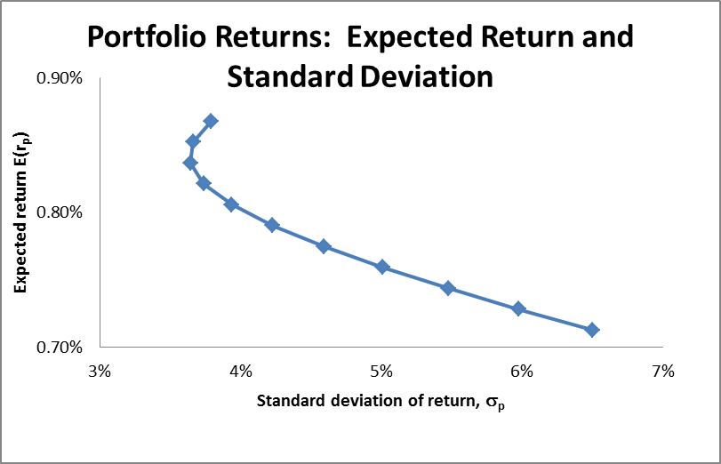
In the graph above, the portfolios that are on the efficient frontier offer a higher amount of return than those that lie in the feasible region. Also, the portfolios on the efficient frontier have a low amount of risk at the same level of return as those that lie in the feasible region.
Minimum and maximum variance portfolios
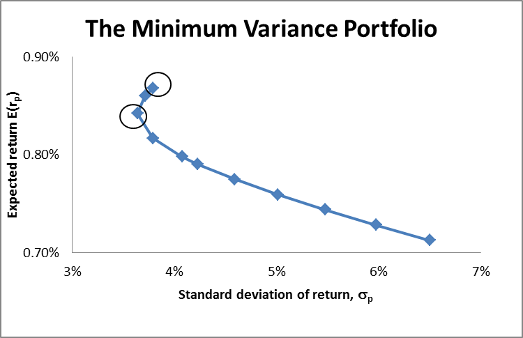
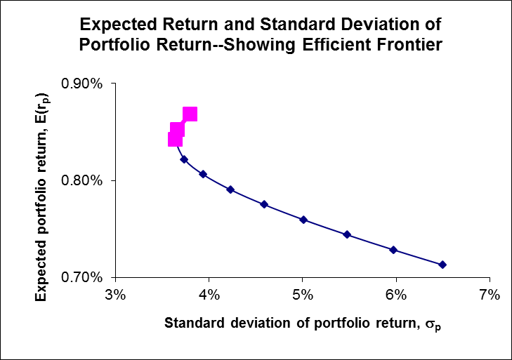
On the efficient frontier presented above, there exists a portfolio that has a minimum risk (as measured by the variance). This point is called the minimum variance portfolio (Elton & Brown 2007). This point is also associated with minimum return. From the calculations presented in appendix 2, the minimum portfolio variance is at the point where the proportion of Proctor & Gamble stock is 83.41%, while the proportion of stock for Royal Bank Canada is 16.58%. The portfolio variance at this point is 3.64%, while the expected return is 0.84%.
On the other hand, maximum variance portfolio is associated with maximum return. In the case of the two companies, the combination that yields this portfolio is by investing 100% in stock of Proctor & Gamble Co. and 0% in Royal Bank of Canada. The resulting value of expected portfolio return is 0.87%, while the variance is 3.79%. The minimum and maximum variance portfolios are illustrated in the graph below.
After locating the minimum and maximum variance portfolios on the frontier, the section of the graph that represents an efficient frontier is presented in the graph below. It is highlighted in pink.
Relationship between correlation and portfolio variance
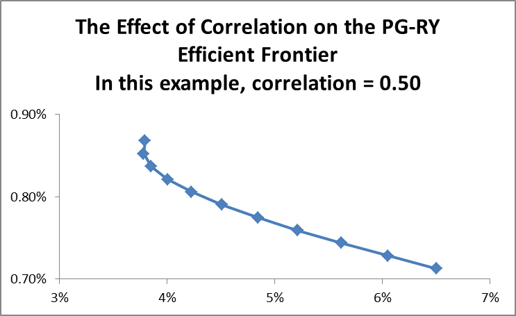
The calculations presented in appendix 2 show that estimation of variance depends on the correlation between the two stocks. Therefore, it is important to analyze how correlation affects the risks of the possible portfolio (Elton & Brown 2007). In this section, the minimum variance frontier will be derived under three different assumptions. In the first case, it is assumed that the correlation coefficient is 0.5. The resulting efficient frontier is presented below.
The second scenario is when the correlation coefficient is 1. The resulting efficient frontier curve is presented below.
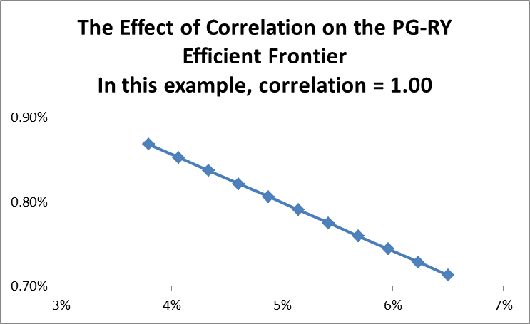
The graph is similar to a scenario where there is one risky and one risk free asset in a portfolio. Since the two assets are perfectly correlated, then it is possible to come up with an artificial risk free asset. Thus, it is possible to form a perfect hedge made up of the two securities. The final scenario is when the correlation coefficient is -1. The efficient frontier curve is presented below.
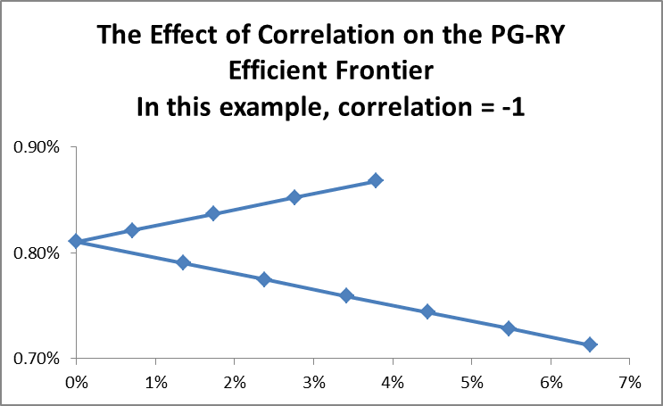
In this case, the two assets are also perfectly correlated and it is possible to form a combination of artificial assets. However, some combinations are dominated.
Systematic and unsystematic risk
Systematic risk is uncertainty that is integral in an entire market. This type of risk cannot be reduced through diversification. Systematic risk is often measured using beta. From the calculations in appendix 3, the value of beta for Proctor & Gamble stock is 0.0163 while that of Royal Bank of Canada is -0.0744. This implies that Proctor & Gamble stock has a lower level of volatility as compared to the market (S&P 500 index) while the stock of Royal Bank Canada has an inverse relation to the market. On the other hand, unsystematic risk is uncertainty that is associated with an entity or the business sector that an individual invests in. This category of risk can be minimized through diversification (Elton & Brown 2007).
Diversification
The concept of diversification is based on the fact that the tradeoff between risk and return improves when an investor holds several assets that have less than perfect correlation. As the number of assets in a portfolio increases, then only the average covariance is significant. This implies that if the average covariance is zero, then the portfolio variance will be close to zero. It is worth mentioning that diversification reduces only the diversifiable risks. These are the non-systematic risks. The non-diversifiable risk remains unchanged. Further, if the covariance of a portfolio is positive, then diversification cannot reduce the risk. This is based on the fact that positive covariance is associated with systematic risk (Elton & Brown 2007).
Central tendency portfolio
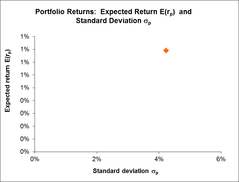
This portfolio is based on the measures of central tendency. The proportion that is used for each stock is 50%. The resulting portfolio mean is 0.79%, while the variance is 0.18%.
Capital allocation problem
There are several approaches that can be used to solve the capital allocation problem. The first approach is based on the Two-Fund Separation theorem. As mentioned above, the second step of this theorem focuses on the combination of risk free asset and the optimal risky portfolio (Elton & Brown 2007). Thus, the portfolio will be expanded to include an asset that has zero risk. The optimal capital allocation, portfolio is obtained by selecting the point of tangency of the capital asset line and the utility function. Therefore, it will be important to come up with the capital asset line and indifference curves. The capital asset line shows all the possible combinations of risk and rate of a return of a risk free and a risky asset. The slope of the capital asset line yields the Sharpe ratio. Therefore, when the two curves are plotted together, the resulting point of tangency gives the optimal level of capital allocation (Elton & Brown 2007).
The second approach of solving capital allocation problem is by using Treynor-Black model. This model seeks to determine the optimal combination of passively and actively managed securities in a portfolio. The model makes use of systematic and unsystematic risk in such a way that assets that have high levels of unsystematic are assigned less weight (Bodie, Kane & Markus 2012).
The first step when using the Treynor-Black model is to estimate the values of alpha and beta of the two stocks. This is carried out using regression analysis. Based on the capital asset pricing model, the values of the rate of return for each stock are regressed on excess return (difference between market rate of return and risk free rate of return). The results of regression are presented in appendix 3 below. The value of alpha for Proctor & Gamble Co. is 0.00848 while that of Royal Bank of Canada is 0.00803. These are estimated values of the Y – intercept.
The next step of the model will be to allocate weights to the stock in the active portfolio. These weights are considered to be directly proportional to the ratio of alpha and unsystematic risks. This ratio is called the Treynor-Black ratio. It gives information on the value that a stock adds to the portfolio on a risk adjusted basis. The allocation will be done in a way that an asset that has a higher level of alpha is assigned higher weight. In the example above, the stock of Proctor & Gamble Co. has a higher value of alpha than that of Royal Canada Bank. Therefore, it is allocated more weight. The results of Treynor-Black model are presented in appendix 3 below.
The results show that the weight for Proctor & Gamble is 75%, while that of Royal Bank of Canada is 25%. The next step is to calculate the weighted averages of the active portfolio. Thus, the beta, alpha and idiosyncratic risk of the active portfolio are -0.00634, 0.00837, and 0.00109. The next step is to estimate the weight of the active portfolio in the overall portfolio. The estimated value of this weight is118.85%. A correction is then carried out to adjust beta of the active portfolio. This ensures that the overall portfolio does not become too risky. It also ensures that there is no variation of portfolio beta of the overall portfolio. The corrected value of beta is 54.12%, while the weight of the passive portfolio is 45.88%. These are optimal weights for the active and passive portfolio (Bodie, Kane & Markus 2012). The calculations of this model are based on the assumption that the security markets are nearly efficient.
Efficient market hypothesis
The theory of efficient market hypothesis holds that all relevant information about the ‘true’ value of an asset that can be found in the market is reflected in its market price. This indicates that a room for arbitrage does not exist in the market (Bodie, Kane & Markus 2012). Thus, if there is information, then it is disseminated and reflected in the prices of stock at a faster rate. This eliminates the possibility of using such kind of information to make gains. An efficient market is associated with the concept of ‘random walk’. Based on the random walk and efficient market hypothesis the stock prices follow a random pattern and future changes in prices cannot be predicted using past data. Thus, future changes in price are independent of previous prices. This is based on the idea that if there is free flow of information, then the information is immediately reflected in the stock prices. Therefore, future changes in prices will only reflect future information and are independent of current changes in price (Bodie, Kane & Markus 2012).
Portfolio valuation and performance (later time frame)
In this section data for the two stocks is collected for the period between 03/3/2013 to 06/3/2014. A summary of the results is presented below.
The information in the table above shows that the expected rate of return of the portfolio for data that is collected after 03/03/2013 is higher than the rate of return for data collected before 03/03/2013. This represents a strong evidence of the efficient market and random walk hypothesis which states that the information on the past trend does not have any relationship with future trends.
Conclusion and recommendations
The discussion above focuses on how to solve the asset and capital allocation problem. An investor is often faced with a challenge of deciding on how to allocate the scarce resources among various securities. Therefore, the discussion above demonstrates how the two problems can be solved. The solution to the asset allocation problem focuses on how an investor can allocate resources between two risky assets. The discussion above indicates that this can be solved by finding a combination of the two securities that yield maximum possible return at a minimum variance. Further, correlation coefficient has an impact on the variance of a portfolio. In the second part, Treynor-Black model is used to solve the capital allocation problem. Based on this model, the optimal allocation of resources is achieved by using systematic and unsystematic risks to allocate weights. The discussion above also shows that the data follow the efficient market hypothesis. Thus, past trends do not have an impact on future trend. As a recommendation, an investor should use various tools of analyzing a portfolio when coming up with the optimal allocation of resources among various securities.
Reference list
Board of Governors of the Federal Reserve System 2013, Economic research & data – historical data. Web.
Bodie, Z, Kane, A & Markus, A 2012, Investments, McGraw Hill Publishing Company, USA.
Elton, G & Brown, G 2007, Modern portfolio theory and investment analysis, John Wiley & Sons Ltd, USA.
Yahoo, Inc. 2009a, The proctor & gamble company (PG).
Yahoo, Inc. 2009b, Royal bank of Canada (RY).
Yahoo, Inc. 2009c, S&P 500 (˄GSPC).
Appendices
Appendix 1 – Data
Appendix 2
Portfolio statistics
Different combinations of assets
Minimum and maximum variance portfolio
Correlation coefficient = 0.5
Possible combinations
Correlation coefficient = 1
Possible combinations
Correlation coefficient = -1
Possible combinations
Appendix 3
Regression results
Proctor & Gamble
Royal Bank of Canada
Results of Treynor-Black model


