Updated:

Analysis for Home Prices for Austin, Texas Research Paper

Exclusively available on Available only on IvyPanda® Made by Human No AI

Introduction

Multiple regression is used to explain situations where several explanatory variables works together to explain a response. In this project, a multiple regression model was used to compare home prices in Austin. Home prices are thought to depend on various independent factors. A sample of about 30 homes in Austin was chosen. A multiple regression analysis was used to determine how various explanatory factors affect the prices of homes in Austin. Multiple regression analysis was used to come up with a regression equation which can be used to predict future home prices in Austin or which can explain why prices for homes in Austin changes from one place to another.

Austin Background

Austin is the capital city of Texas and the seat of Travis County. It is the thirteen most popular city of the United States of America and was among the first three fast–growing cities of USA from 2000 to 2006 (AustinTexas, 2012). The population size of Austin is about 820,611. The city of Austin was started around 1830’s when immigrants settled at the center of Austin. It was made Texas capital by 1839. Initially it was known as Waterloo but the name was later changed to Austin (AustinTexas, 2012).

Austin is a center of high technology and innovation and provides employment for graduates from all over USA. A lot of multinational companies are located in Austin which includes: Dell, Apple, Google, PayPal and Pharmaceutical and Biotechnology. As a result, Austin is a large employment provider for the Americans. Home prices in Austin differ from place to another and the cost is determined by various factors. The cost depends on whether is a single family home, condor or a townhouse. The home prices also depend on their geographical location in Austin, the number of bedrooms and bathrooms present in them and whether the houses contain an attached garage. Last but not least, the home prices are very much determined by the size of the plot where the home is constructed (Zillow, 2012).

Model Specification and Data

The purpose of multiple regression models is to analyse the relation between metric or dichotomous independent variable and a metric dependent variable. Once a relationship exists between the independent variables and the dependent variable, the relationship can be used to predict the values of the dependent variable. The relationship follows the format given below:

Y=β0+ β1x1+ Β2x23x3+ β 3X3 4X4…… βn xK + E

Where

β 0, β 1, β 2, β3 and β4 are parameters

Y= Response or the dependent variable

X1, X2, X3 and X4 are the independent variables/Explanatory variables

Ε= Random error variable/Error term

Values of X1, X2, X3 and X4 are known constants but the values of β 0, β 1, β 2, β3 and β4 have to be estimated to come up with the regression equation. Once they are known one can predict how the independent variables affect the response of dependent variable Y and one can also determine how one independent factor affects the dependent variable as long as the other factors are held constant. For instance, the value of β 1 indicates the change in the mean response per increase in X1 when the rest of the independent variables in the model are held constant.

The parameters β 0, β 1, β 2, β 3 and β4 are frequently called partial regression coefficients because they reflect the partial effect of one independent variable when the rest of the independent variables included in the model are held constant. The value of the error is minimized in multiple regression analysis and the value becomes smaller and smaller as more independent variables are included in analysis (Lind et al, 2012). Regression estimates are more reliable when the number of observations is high or when we have a large data set, when the variance of a given explanatory variable is high and when we have less closely related independent variables.

To analyse home prices of Austin using multiple regression analysis, data was first collected to obtain a representative sample. The data included house types, house plot size in terms of square feet, price per square feet, number of bedrooms present, number of bathrooms present, availability of an attached garage, house views, type of house cooling systems, whether the houses have swimming pools and their location in Austin. All these factors affect the prices of home in Austin making some homes to be costly than others.

The data was obtained online from Zillow, a real estate advertising company using probability sampling whereby a convenient sample was obtained randomly (Zillow, 2012). A sample with a description of 34 homes was obtained which is tabulated in Appendix 1. Four independent variables were selected which include: Square feet(X1), Number of Bedrooms(X2), Number of Bathrooms(X3) and availability of an attached garage (X4) which were subjected to multiple regression model to determine how they affect the home prices for Austin. Once the values of β0 β1, β2 and β3 and β4 were estimated the regression equation was formed.

Presentation and Discussion of Results

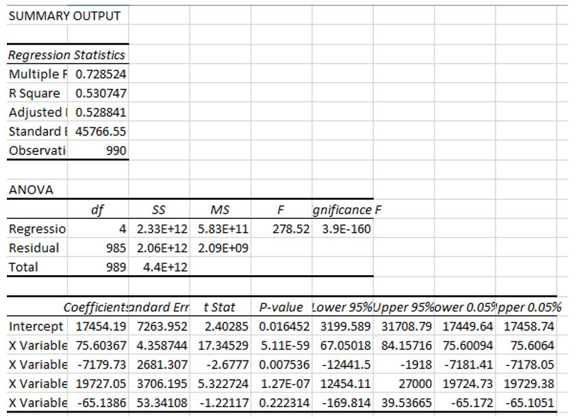
The data in Appendix 1 was subjected to multiple regression analysis using Microsoft excel 2007 data analysis tool. The significance level used in the analysis was 0.05% (Alpha=0.05). The calculated value of R2,adjusted R2, Standard error of the regression coefficient, F statistic and its significance, the values of the parameters (regression coefficients): β0, β123 and β4,standard error of β0, β123 and β4 ,T-test values of the regression coefficients and their significance and well as the 95% confidence intervals for the regression coefficients have been tabulated in Table 1,Table 2 and Table 3 below.

Table 1: Regression statistics.

Regression Statistics.
Multiple R0.811315554Square root of R2
R Square0.658232928R2
Adjusted R Square0.611092643Adjusted R-Squared used for several X’S
Standard Error105815.3112Standard deviation of the regression error (E)
Observations34Total number of observation used in regression (n)

Alpha =0.05

Table 2: Analysis of Variance.

ANOVA
dfSSMSFSignificance F
Regression46.25381E+111.56345E+1113.963278291.82856E-06
Residual293.2471E+1111196880074
Total339.5009E+11

Alpha =0.05

Regression Sum of Squares=6.2538 Regression Mean Square=1.56345E+11

Residual Sum of Squares=3.247 Residual/Error Sum of Squares=11196880074

Total Sum of Squares=9.500 Calculated F=13.9632

Table 3: Regression Coefficients (β0, β1, β2, β3, β4), Standard error of the regression coefficients (Sb0, Sb1, Sb2, Sb3, Sb4), regression coefficient t-values, t-test p-values (test for β0, β1, β2, β3, β4=0) and 95% confidence intervals for the regression coefficients.

Regression CoefficientsStandard Errort StatisticsP-valueLower 95%Upper 95%
Intercept16889.7465970954.263760.2380370920.81352621-128228.0147162007.508
X1(Square feet)144.633824433.120515574.3668953190.0001465976.89476523212.372884
X 2(Bedrooms)-37966.8911333055.33753-1.1485857950.26011288-105572.646329638.864
X 3(Bathrooms)27704.9967834621.055230.8002354810.43008142-43103.0105498513.0041
X4(Garage)51847.4392542007.263421.234249390.22701869-34067.05978137761.938

Alpha =0.05

Y-intercept = β0 = 16889.746. This is the value of Y when all the other variables in the model take the value of zero. The regression equation is given below.

Y = 16889.74+144.634 X1-37966.89 X2+27704.99 X3+51847 X4

HOME PRICE = 16889.74 + 144.634 SQUARE FEET – 37966.89 BEDROOMS + 27704.99 BATHROOMS + 51847GARAGE

As a result, this multiple regression model can be used in predicting interval for a particular value of Y for a given set value of X’s. It can also be used to produce an interval estimate for the expected value of Y for a given set value of X’s. Last but not least the multiple regression model can be used to elucidate the relationship between various explanatory variables and the given independent variable by interpretation of the regression coefficients of the X’s.

Discussion

Adjusted R-squared (R2) represents the proportion of variability of home price explained by the independent variables (X’s). This R2 is adjusted so that models with different number of variables can be compared. R-Squared is used in multiple regression analysis because it does not automatically rise when an extra independent variable is added to the model. However when a new variable is added in multiple regression, it affects the coefficients of the existing variables. Adjusted R2 is dependent on t-statistics of the explanatory variable because when the t-test of an extra variable exceeds 1 the adjusted R2 rises but it does not necessarily imply that the extra independent variable is significant (Lind et al, 2012). From the results in Table1, the adjusted R2 value is 0.6111. This denotes that 60.11% of the total variability of the home prices in Austin, Texas can be attributed to the four independent variables (the regressors) which have been considered in the model.

The F-test shows the analysis of variance of regression and is used to test for the significance of the group of four independent variables used in the analysis. The F-test is a test for goodness of fit of the regression line and it tests for joint significance or restriction of the explanatory variables (Lind et al, 2012). The overall F-statistic from the ANOVA Table 2 is 13.963 and the associated level of significance is 1.828 of H0: β1, β2, β3 and β4 = 0 versus Ha: at least one of β 1, β2, β3 and β4 does not equal zero. The significance value of 1.828 is greater than 0.05 which is the required level of significance. Hence the F statistic value is significant implying that the β1, β2, β3, β4 are not equal to zero. As a result there is a linear relationship between the price and at least one of the four independent variables. This shows that an increase in the number of bathrooms, number of bedrooms and even the plot size will directly cause an increase in home prices in Austin.

The t- test values of each partial regression coefficient have been tabulated in Table 3 together with associated level of significance (p-value) for the four regression coefficients which is 0.0014, 0.2601, 0.4300 and 0.227 for β1, β2, β3 and β4 respectively of H0: β1, β2, β3 and β4 = 0 versus Ha: at least one of β1, β2, β3 and β4 does not equal zero. T-test for β1 is less than 0.05 hence is not significant while t-test for β2, β3 and β4 is significant because it is greater than 0.05. Significant t-test indicates that a given independent variable in the model influences the response of the dependent variable while controlling for the other independent variables (Lind et al., 2012). This implies that factors like number of bedrooms, number of bathrooms and availability of an attached garage to house can individually affect home price in Austin.

Conclusion

Multiple regression models are useful for prediction and forecasting of events such future prices of goods and services with the help of other variables which are likely to affect the prices. Multiple regression models can be used in analyzing seasonal effects whereby F-test is mostly used in making the inferences. Changes in demand and predicting the total production cost of companies for future years can also be achieved by carrying out multiple regression analysis. Multiple regression models are also used in explanation of the current state of situations and even in theory building. In multiple regression analysis, one is interested with the number and significance of relationship between the independent variables and the dependent variable however correlation between variables needs to be considered. This is because in many non-experimental situations such as in business, economic, social and biological sciences, most of the explanatory variables used in multiple regressions are related to themselves.

In this context, multiple regression model can be used tell why the home prices in Austin are differing from one place to another and which factors are positively or negatively influencing the home prices and which factors do not affect home prices in Austin. For instance the price of a single family house with a plot size of 3000 square feet, 5 bedrooms, 3 bathrooms and an attached garage for sell in Austin can be estimated using the regression equation obtained above which will be:

Y=16889.74+144.634 X1-37966.89 X2+27704.99 X3+51847 X4

Home Price in USD = 16889.74 + 144.634(3000) -37966.89(5) +27704.99(3) +5184(1) =$.349, 256.26

References

AustinTexas. (2012). The official Website for the city of Austin. Web.

Lind, D.A., Marchal, W.G. & Wathen, S. (2012). Basic Statistics for Business & Economics.8th edition, Publisher: McGraw-Hill Irwin. Web.

Zillow. (2012). Online Real Estate Advertising Company. Web.

Appendices

Appendix 1: Description of Austin Homes

PRICE(P) IN USDSQUARE FEET(SQFT)P/SQFT IN USDBEDROOMSBATHROOMSGARAGELOCATION AT AUSTIN,TEXASHOUSE TYPE
303,500226413432110309 THISTLE MOSS COVE 78739SINGLE FAMILY(S.F)
219,00017059832113318 PERTHSHIRE ST,78729SINGLE FAMILY(S.F)
280,0002673893318005 WELDON SPRINGS ST.S.F
448,000360110455.502724 COLLYWOOD DR.S.F
210,00096821621.503601 MANCHACA RD APT 106CONDOR( C)
259,90026569742.518822 WHITEWORTH LOOPS.F
139,90013481033211106 JORDAN LNS.F
725,000302323932.513312 WESTHILL DR.CONDOR( C)
124,00010801153106706 TAMPA CV.S.F
180,92019189432014416 LAKE VICTORC
170,0007202361103601 MANCHACA RD APT 111S.F
89,9001049852201015E YAGER LN UNIT 50S.F
99,900135273321901E MENDOWMERE LNS.F
239,900221410832.5010608 DESERT WILLOW LOOPTOWNHOUSE
329,9001741189320400 E 33RD ST.C
635,00026552393311036 LIBERTY PARK DR.#901S.F
165,00017439432.511704 CANNON YEOMANS TRL.S.F
199,90020009942110400 YELLOWSTONE DR.S.F
139,00013001062102731 LYONS RD.S.F
475,00026941764215301 MARSH CREEK DR.S.F
294,00017061723201415 SUFFOLK DR.S.F
400,00018922114311311 PALO DURO RD.S.F
299,000205914532.513007 SUN RIDGE DR.C
124,00088214121.516700 COOPER LN APT 42S.F
549,000316717333111820 GRANITE BAY PIS.F
299,00020591454313007 SUNRIDGE DR.S.F
400,000189221132.511311 PALO DURO RD.S.F
407,00035721134319509 BUNGALOW LNS.F
324,00017801823212202 ALEXANDER AVE.C
350,000352998220804 E 45TH ST.C
114,90010431102211417 W BAKER # BS.F
529,00035021484415732 MISTY HILL CV.S.F
235,00021431094215637 WAGON TRAN RD.S.F
675,000404016744.517201 CERCIS CV.S.F

Appendix 2: Regression statistics, ANOVA, Regression coefficient statistics and Residual output

Regression Statistics
Multiple R0.811315554
R Square0.658232928
Adjusted R Square0.611092643
Standard Error105815.3112
Observations34
ANOVA
dfSSMSFSignificance F
Regression46.25381E+111.56345E+1113.963278291.82856E-06
Residual293.2471E+1111196880074
Total339.5009E+11
CoefficientsStandard Errort StatP-valueLower 95%Upper 95%
Intercept16889.7465970954.263760.2380370920.81352621-128228.0147162007.508
X1(Square feet)144.633824433.120515574.3668953190.0001465976.89476523212.372884
X 2(Bedrooms)-37966.8911333055.33753-1.1485857950.26011288-105572.646329638.864
X 3(Bathrooms)27704.9967834621.055230.8002354810.43008142-43103.0105498513.0041
X4(Garage)51847.4392542007.263421.234249390.22701869-34067.05978137761.938
RESIDUAL OUTPUT
ObservationPredicted Y(Price)ResidualsStandard Residuals
1337697.4845-34197.48447-0.344749479
2256847.1766-37847.17663-0.381542521
3424557.7154-144557.7154-1.457305935
4500259.1749-52259.17493-0.52683183
5122519.001587480.998470.881907811
6370279.5509-110379.5509-1.112751223
7205212.9013-65312.90131-0.658428216
8461327.0556263672.94442.658122714
986898.6003437101.399660.374024242
10235806.742-54886.74198-0.55332069
11110764.205859235.794180.597164075
12148086.8397-58186.8397-0.586589423
13205791.4366-105891.4366-1.067505934
14292470.8524-52570.85239-0.529973893
15210206.5551119693.44491.206645852
16421954.3066213045.69342.14774253
17276195.7603-111195.7603-1.120979541
18261547.2637-61647.26369-0.621474426
19156684.9328-17684.93284-0.178284207
20361923.1378113076.86221.139943184
21205144.371288855.62880.895765645
22273631.8074126368.19261.273934888
23321900.0489-22900.04886-0.230858498
24161927.9319-37927.93188-0.382356625
25496006.824752993.175310.534231388
26297785.65611214.3438830.012241965
27297746.2002102253.79981.030834425
28516616.6324-109616.6324-1.105060139
29267694.713556305.286540.56762123
30506778.7242-156778.7242-1.580507583
31199066.476-84166.476-0.84849366
32534197.2615-5197.261516-0.052394298
33282229.9006-47229.90058-0.476131034
34625862.757449137.242560.495359207
More related papers Related Essay Examples
Cite This paper
You're welcome to use this sample in your assignment. Be sure to cite it correctly

Reference

IvyPanda. (2022, May 3). Analysis for Home Prices for Austin, Texas. https://ivypanda.com/essays/analysis-for-home-prices-for-austin-texas/

Work Cited

"Analysis for Home Prices for Austin, Texas." IvyPanda, 3 May 2022, ivypanda.com/essays/analysis-for-home-prices-for-austin-texas/.

References

IvyPanda. (2022) 'Analysis for Home Prices for Austin, Texas'. 3 May.

References

IvyPanda. 2022. "Analysis for Home Prices for Austin, Texas." May 3, 2022. https://ivypanda.com/essays/analysis-for-home-prices-for-austin-texas/.

1. IvyPanda. "Analysis for Home Prices for Austin, Texas." May 3, 2022. https://ivypanda.com/essays/analysis-for-home-prices-for-austin-texas/.


Bibliography


IvyPanda. "Analysis for Home Prices for Austin, Texas." May 3, 2022. https://ivypanda.com/essays/analysis-for-home-prices-for-austin-texas/.

If, for any reason, you believe that this content should not be published on our website, please request its removal.
Updated:
This academic paper example has been carefully picked, checked and refined by our editorial team.
No AI was involved: only quilified experts contributed.
You are free to use it for the following purposes:
  • To find inspiration for your paper and overcome writer’s block
  • As a source of information (ensure proper referencing)
  • As a template for you assignment
1 / 1