Custom Random Number Generator Essay

Introduction

An integer can be generated randomly using a computer program known as custom random number generator. It generates a random number between two chosen integers. Two integers are keyed in depending on the desired interval (Glosser, 1998). The number is generated in a predictable manner and is pseudo random in nature (Pseudo-random numbers, n.d.). The generated random number is 3.

Starting with the 3^rd piece of data, systematic sampling was used and the subset of data selected is shown in table 1 below.

Table 1: Systematically sampled subsets of data.

Systematic sampling involves choosing a starting number at random and thereafter at regular intervals determined from the generated random integer. The samples are 100 dividing by the random integer 3 gives 33.3, so every third applicant is chosen starting from the 3^rd applicant. Therefore, the subset data generated is of 33 applicants.

Mean, median, mode calculations

Determining mean, median and mode

The summation of the two data sets is obtained

For unsuccessful applicants, ∑ = 1440

Mean = total age of applicants/Total number of applicants

= 1440/33 =43.64 yrs

For successful applicants, ∑=1312

Mean=1312/33 =39.75yrs

The median is the middle number of the data set. Arranging in ascending order, the median is found.

For unsuccessful applicants, median =44 yrs

For successful applicants, median=39 yrs

The mode is the number occurring most often in the data set.

For unsuccessful applicants, mode=37yrs

For successful applicants, mode=39yrs

Determining range and standard deviation

The variance =∑(xi-x’)^2/n where xi is the ith element in the data set, x’ is the mean and n is the total number of the data.

For unsuccessful applicants

Table 2: Variance table for unsuccessful data subset.

Variance =1711.636364/33 =51.867

Population Standard deviation σ=√variance =√51.867 =7.20

The sample standard deviation S=√(X-X’)/n-1

S=√1711.6363/32=7.31359

The range is the difference between the lowest and highest values in a data set. For unsuccessful applicants, the range=57-29=28yrs.

Successful applicants

Table 3: Variance table for successful data subset.

Variance =768.0606061/33=23.274

Population standard deviation=√23.274 = 4.824

The sample standard deviation S=√(X-X’)/n-1

S=√768.0606/32=4.8991

Range=51-33=18yrs

Results table

Table 4: Results table.

The two sets of data have their mean, median and mode centered around 37-44yrs. We have many older applicants in the unsuccessful group as compared to the successful group. This can be seen from the wide range obtained (28yrs) and the mean age of 43.64. The ages for the unsuccessful group deviate from the mean by a very wide margin of 7.31359. The successful group is mostly centered around 39yrs with less deviation 4.8991 from the mean.

Graphical representations

Histogram representations

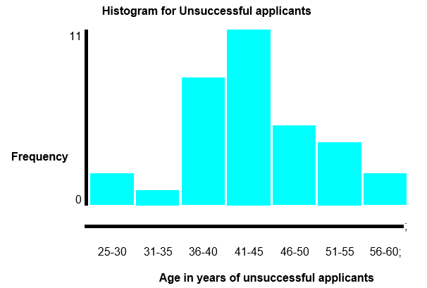
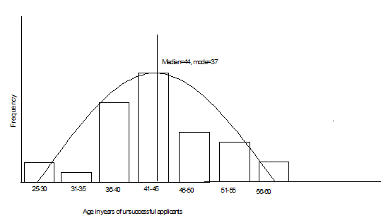
The median is 44, mode =37 and mean is 43.64.

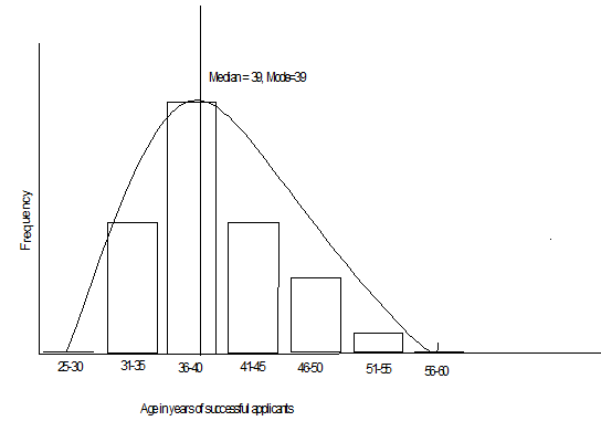
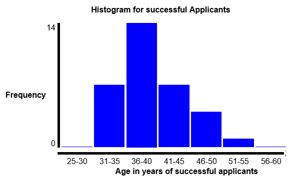
The median is 39, mode =39 and mean is 39.75.

Constructing box plots

Unsuccessful applicants

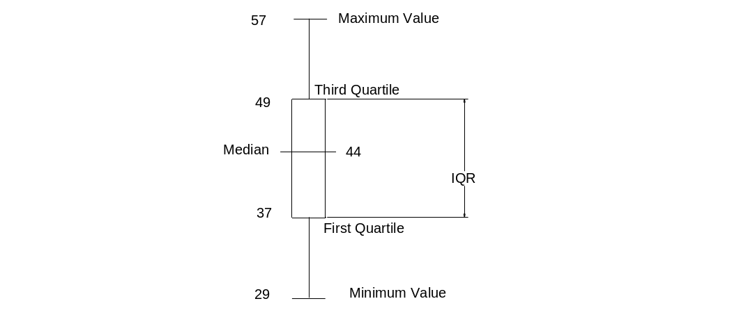
Maximum value=57yrs;

Minimum value=29yrs;

Median=44;

1^st quartile=37;

3^rd quartile=49;

Inter quartile range=49-37=12;

Upper fence for outliers=3^rd quartile+1.5IQR= 49+ (1.5*12) =67;

Lower fence for outliers=1^st quartile-1.5IQR=37-(1.5*12) =19;

Therefore, there are no outliers.

Successful applicants

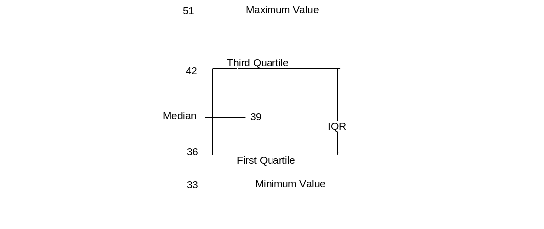
Minimum value=33;

Maximum value=51;

1^st quartile=36;

Median=39;

3^rd quartile=42;

Inter quartile range=42-36=6;

Upper fence for outliers=3^rd quartile+1.5IQR= 42+(1.5*6)=51;

Lower fence for outliers=1^st quartile-1.5IQR=36-(1.5*6) =27;

The data value 51 is on the border. Therefore, there is no outlier.

Histograms and box plots help in showing the distribution of the data sets. The histogram for unsuccessful applicants shows a normal evenly distributed population (bell shaped) on both sides. This implies the age of the unsuccessful applicants is balanced about the central point (median). The histogram for successful applicants is skewed towards the right. This implies that the age of successful applicants is unbalanced about the central point (median = 39) but its distribution is near a normal distribution. The box plot for unsuccessful applicants shows an even distribution of the whiskers meaning its population is evenly distributed while that for successful applicants is uneven. The lower and upper quartiles have 25% of lower and upper values respectively.

Formulation of hypotheses

The hypotheses will test whether the means are different. The hypothesized mean is 40 yrs. The null hypothesis will determine whether the sample means of both samples are equal, unsuccessful applicants mean μ1=successful applicants means μ2, such that the means of the two groups are not significantly different.

• Null hypothesis Ho: μ1=μ2
• Alternate hypothesis H1: μ1≠μ2 (two tailed test)

The alpha level represents the significance level of the hypothesis. It gives the probability of rejecting the null hypothesis when it is true (type 1 error), that is, it is the probability of concluding that the research hypothesis is true when the null hypothesis is true. When the p-value is less than 0.025 for a two tailed test, the null hypothesis is rejected.

The z statistic will be used for hypothesis testing. The population size is large at 33 (n˃30) and the population standard deviations are known.

The z statistic is

where x bar is the sample mean of unsuccessful and successful applicants, σ is the standard deviation and n is the sample size.

The Z value is given as Z=43.64-39.75/√(7.31359²/33⁺4.8991²/33)=1.6566.

The shaded region below is the rejection region R.

Rejection region R: Z˃1.96 and z<1.96

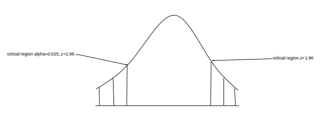
Since 1.6566 <1.96, we accept the null hypothesis. This means the means of the unsuccessful and successful groups are not significantly different.

The null hypothesis is not rejected. This implies that the means of the two groups is not significantly different. The mean age of the unsuccessful applicants is 43.64 while for successful applicants is 39.75.

Confidence intervals

Margin of error

Margin of error m= mean ± standard deviation

For unsuccessful group, margin of error m= 43.63±7.31359

M=36.31 to 50.94

For successful applicants, the margin of error is M=39.75±4.8991=34.85 to 44.64

At 90% confidence level, the critical value is 1.64 which is calculated from (1-0.9)/2=0.05 and looking it up the z value from the table.

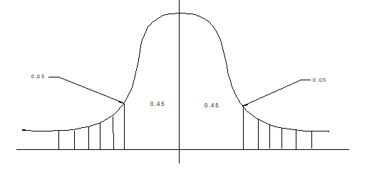
Desired confidence interval

The difference of means x1-x2=43.64-39.75=3.89

Standard error of the difference=√(σ1²/n1+σ2²/n2)=√(7.313²/33+4.8991²/33)=1.5313

CI=X1-X2±1.64*1.531.

CI=3.89±2.51=1.38 to 6.4.

Confidence intervals are signs of estimates reliability. The two data samples have been sampled from a larger group of data. The confidence interval shows how frequently a particular unknown parameter is included in an observed interval.

Conclusion

From the graphical representations and after hypothesis testing, it was found that the mean age for unsuccessful applicants was 43.64 yrs while that for successful applicants was 39.75. The margin of error for both data sets is small. The confidence interval for the group is 1.38 to 6.4. This means that the sampled population is highly reliable in giving the correct results. The histograms and box plots portray a near normal bell shaped distribution. It can be safely concluded that there is no discrimination in the selection. Since sampling was done, it is assumed that the whole population will present an almost equal result or improve on the result hence the hiring process can be retained.

References

Glosser, M. G. (1998). Custom random number generator. Web.

Pseudo-random numbers, (n.d.). Web.