Abstract
This report is about use of Factor analysis especially using SPSS to analyze a very large data set and to see if there is any correlation between the data. Simply, factor analysis encompasses creation of a single or several hidden independent variables, which associate with the observed data. This process is known as a technique for data reduction. If they exist how they are correlated is the main aim of this study. Using random.org, I generated 4900 random numbers ranging from 1 to 100, arranged in seven columns. To use factor analysis to determine the nature of the underlying relationships, we have to use this set of random data as our data are set in SPSS. So, the next step was to transfer the random numbers to SPSS to enable the analysis. The random data have been attached.
It can be assumed that the seven columns are seven variables of a given case (row), i.e. test scores of say 700 students. As psychologists, we want to find out if the test scores of some of the tests depend on some of the other test scores of other subjects. In my analysis, I first did the extraction of data before doing the final rotation to obtain the require correlation matrix which has the coefficients indicating the strength of correlation between the test variables.
In my case, I decided to determine if the test score of the first variable (test score of first subject) measured variable is correlated to the 2nd and 3rd test scores and so on until the 7th test score for all the seven hundred whose scores were used in the analysis and make a conclusion.
I developed the hypothesis that the scores obtained by each student are dependent on the scores of the other subjects (6).
Two stages are involved in factor analysis:
- Factor extraction.
- Factor rotation.
Factor Extraction helps identify the amount of highlighted factors. A screed plot is also used in the analysis to show graphically the relative values of the Eigen values. Eigen values indicate the number of rotation in a set of measures that a specific factor signifies. In our analysis, we were able to extract 3 components, i.e. three components had an Eigen value greater than after performing the extraction procedure. The last stage involves examination of the patterns of correspondence in the factor of the rotation matrix of a unit output (StatSoft n. d.). The maximum iterations before convergence are set to 25.
Introduction
The main aim for this task is to determine if one can analyze a given large data set to see if he/she can find out any underlying factors in the data. Since there was no data available, I was asked to generate 4,900 random numbers from the website www.random.org. With the generated random numbers, I exported them first to excel before exporting them finally to SPSS for easier analysis to determine the underlying dependency.
Factor analysis shrinks and evaluates large sets of data to establish fundamental factors and evaluate their effects on variables set (Random.org). Surveyors often employ factor analysis to identify undetected factors that impact responses survey questions. These professionals employ statistical software such as SPSS to conduct this complex computation. IBM Company is the custodian of SPSS. The software guides the user through some basic steps necessary to finish the key stages of factor analysis, including factor extraction, and factor rotation (Random.org).
Extraction facilitates the identification of the numerals of fundamental factors. The user does extraction process by looking at two output parts at this level, which are the screen plot and the initial Eigen values. Eigen values indicate number of rotation in a set of measures that a factor defines. It is wise to include all factors with Eigen values greater than 1. The screen plot on the other hand is a graph of the Eigen values against the components (factors). All factors with Eigen values greater than 1 are to b retained. Rotation works these factors into more meaningful elements. From SPSS, I did the Factor analysis so as to come up with the following work.
Analysis
After generating the random numbers and saving them as a.sav file (SPSS file format), the analysis began. After accessing the data file select Analyze, then click on either “Data Reduction” or “Dimension Reduction”. These alternatives are a factor of the SPSS version of the user. Then select “Factor Analysis” (a factor analysis dialogue box opens). Subsequently, the user chooses the variables that he or she wants to conduct the analysis and move the variable by clicking an arrow key into a variables box. Further, select “Extraction” in the dialogue box of factor analysis (Jaccard and Becker 2001).
The dialogue boxes states that SPSS applies the procedure of principal part factors analysis mines Eigen measures that are greater than 1 and showing a solution of unrotated factor. Click “Continue” to return to the factor analysis dialogue box. Consequently, select “OK” in the dialog box of factor analysis. SPSS output the results of the analysis in an output file, explained in the subsequent lines. From the results, it was noted that there are 3 components which had an Eigen value greater than 1 and with these 3 components. I proceeded to do the factor rotation analysis whose procedure is outlined below:
Click “Analyze” then select “Data Reduction” followed by “Factor analysis”. Then Click “Extraction” and in the extraction dialog box under extract, select the “Number of factors” option and then type the number of factors to rotate (StatSoft n. d.). I chose to be equal to 3 because only three components had an Eigen value greater than 1. Then click “Continue” to return to the factor analysis dialog box. Click “Rotation” I chose Varimax as my method of rotation. This method usually analyses the variables and underlying factors (Jaccard and Becker 2001).
After performing the initial Factor extraction, the following results were obtained as shown (Jaccard and Becker 2001). The correlation matrix is as shown in figure1. From the table, it can be seen that very small correlation between the data (in our case the assumed test scores). For instance, the correlation between component 1 and component 2 IS -.054 which signifies a weak inverse relationship between the two variables.
The correlation between component 1 and component 3 IS -.039 which signifies a weak inverse relationship between the two variables. The correlation between component 1 and component 4 IS -.028 which signifies a weak inverse relationship between the two. The correlation between component 1 and component 5 IS -.043 which signifies a weak inverse relationship between the two variables. The correlation between component 1 and component 6 IS -.014 which signifies a weak inverse relationship between the two variables (Jaccard and Becker 2001). The correlation between component 1 and component 7 IS -.046 which signifies a weak inverse relationship between the two variables.
The correlation between component 2 and component 3 IS -.010 which signifies a weak inverse relationship between the two variables (Jaccard and Becker 2001). The correlation between component 2 and component 3 IS -.038 which signifies a weak inverse relationship between the two variables. And the rest correlation can be interpreted similarly from the correlation matrix given below.
Figure 1.
Figure 2.
Variances between the variables are given by the following figure 3.
Of all the seven underlying factors their initial Eigen values and their corresponding variances are shown in the table above. It is a summary of their analyses of variances. Figure3
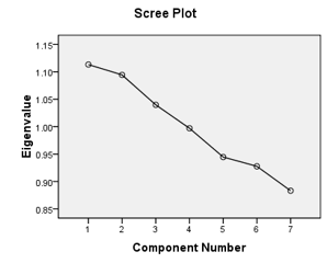
The Scree plot for the data is given in figure4.
From the plot the only component to be extracted are components 1, 2 and 3 since they all have Eigen values greater than 1. So they are the ones we will proceed with to the next stage of analysis.
From the table the components to be extracted are the ones with the Eigen values greater than 1. These components are: 1, 2 and 3.
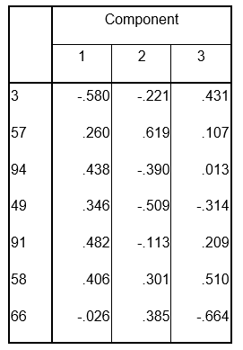
The extracted component matrix is:

Extraction Method: Principal Component Analysis
The results obtained after Factor rotation stage show that the three components depend on some underlying factor with a value greater than absolute 0.3 as shown below:. Component three was discarded due to low factor loadings so that, at the end, we have only two components (StatSoft n. d.).
Conclusion
From the given set of data after the analysis, there is a relationship between the components 1 and 2 and the 3 variables. It can be determined that there were 3 underlying factors in the data set which were previously not considered or are unknown. So, the necessary steps are to be taken to get the exact impact of the underlying factors. The rotation also converged only after 3 rotations although the procedure permits up to 25 rotations.
References
Jaccard, J., & Becker, M. A. (2001). Statistics for the Behavioral Sciences. (5th Ed.).
Random.org. (n.d.). Web.
StatSoft. (n.d.). Principal Components and Factor Analysis. Web.