Introduction
The eternal quest to predict future events has spilled over into the investigation of reliable techniques for predicting the movement of financial markets, particularly with a view to optimizing returns. Since the 1960s, much attention has been given to testing Eugene Fama’s Efficient Market Hypothesis, which the author posits in three forms: weak, semi-strong and strong forms. The latter postulates that historic information can substantively forecast future security prices and hence, composite indices (CI’s). Given this view, financial analysts have rightly moved toward linear regression modelling to forecast the state of CI. (Simon, 2005).
The purpose of all multiple regression works is to predict a criterion variable better. In this case, an investor who presumably wishes to put some money in an index fund is faced with a great deal of uncertainty about how the composite index will behave. But if there were firm indicators for how the chosen independent variables might behave, then it might be possible to position a fund in long or short positions.
Methodology
Develop a multiple regression model which could be used to predict the composite index from Stock Volume, Reported Trades, Dollar Value and Warrants Volume.
In Minitab 15, load datafile “Stock_Market.MPJ”. Next trigger the command sequence Stat-Regression-Regression. In the menu, type in, or transfer ‘Composite Index’ to the ‘Response’ box. Tab to ‘Predictors’ and choose (or type in) the assigned independent variables (IV’s): Stock Volume, Reported Trades, Dollar Value and Warrants Volume. Choose all necessary diagnostic options in the sub-menus
Findings
The Long-term Market Trend
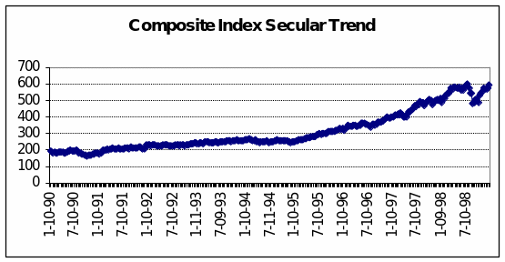
Over most of the decade, the Composite Index for this stock market exhibited a slowly rising trend. An investor who had put in a thousand dollars in an Index Fund on January 10, 1990, would have realised little more than a doubling of his investment (+108.6%) by the same date in 1997. This represents an average annual growth rate of 15.5% in capital appreciation (Fortune, 1998).
Thereafter (see Figure 1 overleaf), activity in the market picked up and the CI reached a high of 599.21 on July 20, 1998. A long correction followed but by the end of the time series, the market had essentially returned to that decade-long high.
The Derived Multiple Regression Model
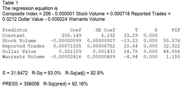
This prediction model is best-understood component by component. The first but least important is the initial number on the right-hand side of the equation, 206. This is technically known as the “intercept”, the starting point for the prediction line if one were to chart the result of the prediction model. This is the value on the Y axis, meaning that over the time period for which there is data, the stock market Composite Index takes a value of $206.15 (see also the first value Minitab reports in the ‘Coef’ column above) if none of the independent variables were in effect. In short, one may consider the intercept as something akin to a ‘base value’ in this analysis. Another way of coming to grips with the concept is to notice that the long-term trend depicted in Figure 1 starts at just under $200. If none of the predictor variables acted on the criterion variable, the chart would show a flat line at $206. across the whole time period.
The second point worth noting is that the prediction model contains a mix of plus and minus signs. This combination reveals that the activity of the Composite Index is directly proportional to the number of trades executed and their aggregate dollar value but inversely proportional to the volume of stocks and warrants that were bought/sold that day.
And the third, most important piece of information is embodied by the ‘beta coefficients’, the values associated with each predictor variable. These tell us that, taken together:
- An increase of 0.000718 standard deviations in ‘reported trades’ for the day will lead to an increase of 1 SD in the criterion variable.
- Similarly, an increase of 0.0212 SD in the dollar value of all trades for the day should boost the entire composite index by 1 SD.
- These beta values look deceptively small and inconsequential until one remembers that the average volume of trades reported during this analysis period was in the order of just under a quarter of a million daily whilst the dollar values averaged $12,968 (this is likely in thousands of dollars) and in fact routinely stood at double that average by the end of the reference period. Hence, the composite index responds substantively to small changes in the number of trades executed and especially to stock prices.
- In turn, the composite index is inversely related to the volume of stocks and warrants traded that day. Specifically, an increase of 0.000001 SD in Stock Volume and 0.000024 SD in the volume of warrants traded depresses the Composite Index one SD.
Another way to understand the results of this analysis is, of course, to recall just what composes a stock market composite index. Every index comprises selections of the stocks in that market – some on an empirical, ‘market-making’ basis and others that are judgment calls because their movements have a disproportionate influence on the movement of the market as a whole. The stock price is a core component of all indices and so is volume.
Why should the volume of “product” traded at the exchanges – stocks and warrants both – depress the Composite Index and hence, contribute to a ‘bear market’ in the making? While everyone knows what stocks are, insight into this question is sharpened by knowing what warrants are.
A stock warrant is a derivative granting the holder ‘the right to purchase securities (usually equity) from the issuer at a specific price within a certain time frame…the main difference between warrants and call options is that warrants are issued and guaranteed by the company, whereas options are exchange instruments and are not issued by the company. Also, the lifetime of a warrant is often measured in years, while the lifetime of a typical option is measured in months’ (Forbes/Investopedia LLC, 2009). For all practical purposes, therefore, the typical stock warrant is equivalent to regular stock.
The logical explanation for the inverse relationship of stock and warrant volume to the CI is that both reflect a flood of ‘sell’ orders hitting the market. On the other hand, the positive relationship between reported trades and the CI shows the repercussion of ‘buy’ orders that not only match but even exceed ‘sell’ for that day. News about favourable macroeconomic indicators or corporate performance itself lifts expectations about capital appreciation to be had and individual stock prices consequently rise. There need not be very many such ‘buy’ orders but the number of completed trades has a positive impact on a price-based index.
Diagnostics
How well does this predictive model stand up to the standard indices of reliability and explanatory power?
First of all, there is R, the correlation between the observed value and the predicted value of the criterion variable. The computed value for Pearson’s R (0.96, not shown in Table 2 overleaf) shows a near-optimal fit between the actual and predicted levels of the composite index.
R Square (R2), shown in the Minitab model summary (Table 2 below), is the square of R and reveals the proportion of the variance in the criterion variable accounted for by all four variables incorporated in the model. Thus, Stock Volume, Reported Trades, Dollar Value and Warrants Volume together account for 93% of the variance in the CI over time.
R2 is a fundamental and widely-cited measure of how good the prediction of the CI criterion variable becomes as long as we have reliable information on where the predictor variables are headed.
However, R2 is prone to slightly over-estimate the success of the model when applied to ‘real-world’ rigour (Gujarati, 1999). Hence, Minitab also calculates an ‘Adjusted R2 value to account for the number of variables in the model and the number of observations (years) the model is based on. At 92.8%, the Adjusted R2 value renders the reliable measure of the success of the model. In this case, we are more confident that the model has accounted for 93% of the variance in the criterion variable. This measure of the strength of the relationship between the actual CI and the predicted CI is called ‘multiple correlation’.
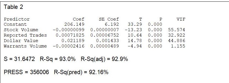
Given the beta coefficients and the standard error for each, we can derive the 95% confidence interval via: β ± (1.96*SE). Following these, we derive the intervals below with only a 5% chance that we are wrong:
Stock Volume = -0.0000011272 to -0.0000008528
Reported Trades = 0.0005859108 to 0.0008505892
Dollar Value = 0.0183803200 to 0.0239976800
Warrants Volume = -0.0000337444 to -0.0000145756
By way of example, we state that every additional thousand dollars entering the market that day adds between 0.018 to 0.024 to the Composite Index.
A second major concern in model diagnostics is parsimony. That is, does the predictive analysis include as few predictor variables as possible by eliminating those that are highly correlated with each other? This is known as testing for collinearity.
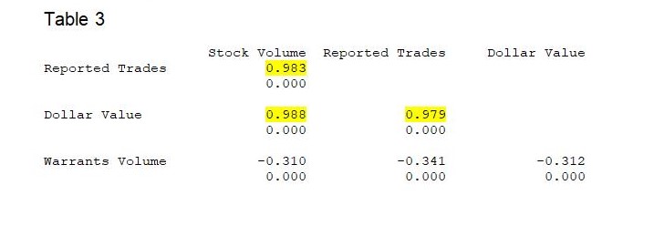
The concern with collinearity springs from the intercorrelation findings (Table 3 above) that Stock Volume is highly correlated with Reported Trades and Dollar Value. In turn, Reported Trades itself is strongly correlated with Dollar Value. Note that the correlation of each predictor with the residuals or error values is 0, which is as it should be.
Other measures for detection of multicollinearity, as suggested by Gujarati (1999, 322) are:
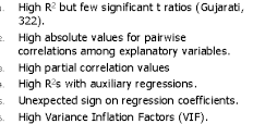
If none of the 6 items are detected, there should not be any multicollinearity in the model. But multicollinearity is a strong supposition if at least one of the 6 items is found.
For the first test, Table 2 affirms that R2 is very high but all the t ratios are in fact significant at p < 0.001. On the other hand, the model fails the test of ‘High partial correlation values: abs (pcv) > 0.9’. All the partial correlation values in Table 3 (except those involving Warrants Volume) are extremely high and turn out to have absolute values ranging from 0.979 to 0.988. Thirdly, all the Variance Inflation Factors (VIF’s, see Table 2 above) except for Warrants Volume are greater than 2. Fourth, one concedes that there are unexpected signs in the model coefficients. It does take some convoluted reasoning to rationalise why the signs for both Stock and Warrant Volumes are negative.
Table 4-1
One, therefore, concludes that the model contains multicollinearity. Refining the model to eliminate these will require eliminating at least one of the predictive variables, retesting on more recent periods or for a new sample from another stock market, reconceptualise the model, restudy the literature to gain new insight on other predictor variables, or transforming the variables (Gujarati, 331-334).
Continuing with diagnostics for this regression model, we see from the Analysis of Variance section of the output that at 4 degrees of freedom, the computed F value is 1,014.16 (see Table 5 below). An F value of this magnitude can occur by chance less than five times in a thousand sampling runs of stock market activity. Hence, we conclude that the model permits predictions of extremely high confidence.

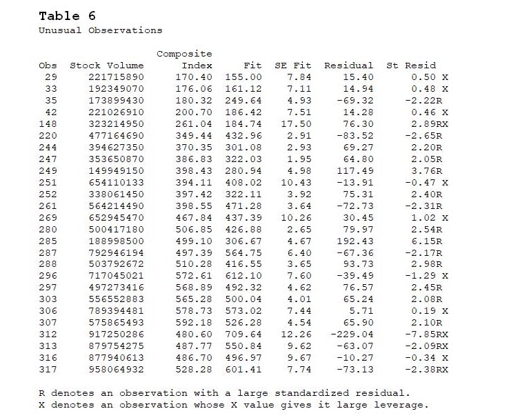
Next, the program identifies 26 cases with large standardized residuals (see Table 6), alluding to large differences (‘outliers’) between the actual and predicted values of the CI. The 35th observation is a case in point: the standardized residual of -2.22 (rather lower than it should have been) is a red flag for looking at the data point more closely. Perhaps, there was some unusual event that took place then.
There are also eight ‘influential cases’, marked with an X. Case 249, for instance, can be considered more important than the others in determining the values of the coefficients. Again, the existence of this ‘outlier’ bears some investigation as this might yield some real-world event that has a bearing on refining the model later on.
Parenthetically, one notes that there are 4 special cases that both display large standardized residuals and appear to have unusually strong leverage on the model results.
A third diagnostic available in the multiple regression model is the Durbin- Waston test, employed to test the hypothesis that the autocorrelation parameter, r, is zero. Specifically,…

versus (for positive autocorrelation)

For the number of predictor variables k = 4 and n observations ≥ 200 (there are 324 data points in the time series tested), the standard table for the Durbin-Watson Statistic at 5 Per Cent Significance Points of dL and dU provides hurdle values of 1.728 and 1.809 for dL and dU, respectively. Since the calculated Durbin-Watson statistic = 1.67521 is lower than the dL value, we conclude that the autocorrelation coefficient is positive and reject the null hypothesis. There is autocorrelation in this time series: a stock market Composite Index behaves according to prior states of the market.
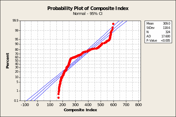
Lastly, one checks the model based on the ‘four-in-one charting’ facility available in Minitab. Were the residuals normally distributed, the Probability Plot of the Composite Index should show all the red (computed CI) points very close to the blue line and an overall shape resembling a normal distribution (Figure 2 below). But there are evidently cyclical forces at work and observations that stray from the blue line plotted. For instance, Minitab flags observation #28, that for October 10, 1990, that is 22.5% below what one would expect if the predictor variables chosen perfectly explained all instances of the Composite Index.
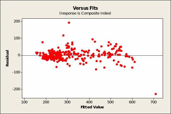
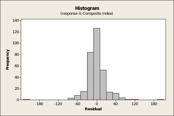
The residuals versus fitted values (Figure 3 below) show, as expected, randomly scatter, true except maybe for the case at row #285 (November 28, 1997) with a FIT2 value of 306.7 and a RESI2 result of 192.4. That the model is robust is shown by the finding that the histogram of residuals (Figure 5 overleaf) shows a normal distribution.
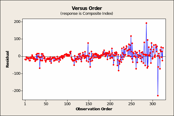
In turn, the observation order chart (Figure 4 on the prior page) is a critical diagnostic only if the order of observations in the dataset has some meaning. While this is technically true for time series data, the presumption is that the information was gathered from a stock market archive at the same point in time.
Conclusions
The choice of four predictor variables from the database – Stock Volume, Reported Trades, Dollar Value and Warrants Volume – to predict the Composite Index has yielded both strengths and vulnerabilities. On the plus side, the model-selected variables explain a great deal of the movement (or variance) over time of a stock market CI. On the other hand, there is autocorrelation and multicollinearity.
Recommendations
Any effort to improve the probability of capital appreciation by investing in a composite index fund or simply predicting with greater confidence how ‘the market will behave’ tomorrow or next week may start with this model. However, refinements are necessary, notably in respect of testing for lagged effects and reducing the set of predictor variables that are move in tandem: Stock Volume, Reported Trades, Dollar Value. It is also vital to reassess the role of Stock Warrants which this initial analysis demonstrated to have an inverse relationship.
Bibliography
Forbes Magazine/Investopedia LLC (2009) Warrant [Internet] Web.
Fortune, P. (1998) A primer on U.S. stock price indices. New England Economic Review, 1998, pp. 25-40.
Gujarati, D. (1999) Essentials of Econometrics. 2nd ed. Boston, Irwin/McGraw-Hill.
Middle Tennessee State University (n.d.) Stats @ MTSU [Internet]
Simon, Helen K., D.B.A. (2005) An examination of the weak form of the Efficient Market Hypothesis within the context of the NASDAQ Composite Index: A test of the forecasting abilities of artificial neural networks. Ph. D. dissertation, Nova Southeastern University.