Introduction
The term microeconomics is derived from the Greek word mikros which means small. Therefore, in microeconomics, the focus is on individual economic units such as individual consumer or an individual firm or an individual factor owner. Each of these small units seeks to maximize or minimize something (Mukherjee 2007, p. 33).
Normally, microeconomics consists of looking at the economy through a microscope, as it were, to see how individuals or households as consumers, and the individual or firms as producers, play their part in the working of the economy.
In general, microeconomics concerns itself with the explanation and analysis of how the various cells of the economic organism or the so-called units of economic such as millions of consumers, producers or business firms, workers and factory owners perform their economic activities and succeed in reaching their respective equilibrium states or achieving their optimization goals such as utility maximization, profit maximization, or optimization of incomes.
This paper presents a discussion of two issues related to the subject of microeconomics. First, the main economic factors that determine the price of a good or service will be explained and later, economic factors that have led to the rises in the prices of cereals in the past five years will be examined.
Factors that Determine the Price of a Good or Service
Two main factors that directly influence the price of goods or services in the market are demand and supply. Generally, the price of goods and services is high when the demand is high (Grant & Vidler, 2000).
A low demand on the other hand implies that the producers have no choice but to reduce the prices as the competition to sell is high and the focus for each seller is to be able to attract as many buyers as may be practically possible.
This, however, typically applies in a free market economy where the prevailing market conditions determine the prices. In a similar way, low supply will result in high prices for goods or services while a high supply will mean that prices have to go up (Mukherjee 2007, p. 35).
According to Odland (2012, p. 1), the price of goods and services is considered a function of both supply and demand.
The effects of demand and supply on the price of a good or a service are explained in the following sub sections.
Demand
Demand relates to the behavior of consumers. The quantity demanded of any good or service is the amount of the good or service that buyers are willing to and able to purchase (Jones 2004, p.64).
Although there are many things that determine the price of a good or service, the level of demand for the good or service affects the price that sellers can offer. Ideally, when the demand is high, the price tends to go up. Regardless of what is responsible for causing the increase in demand, the consumer will be expected to pay a higher price.
The demand may rise due to an influx of people into the market, artificial shortages created by suppliers, or poor infrastructure making it difficult to deliver the good or service as expected (Mankiw & Taylor, 2006). As an example, consider how the cost of fuel keeps fluctuating in many countries across the world.
Usually, the demand of fuel may increase as a result of war experienced in oil producing countries or it may be caused by increased activities such as during Christmas or during Easter celebrations.
Given that the same commodity is being sought after by a higher number of people, it is most likely that sellers will take advantage and start selling the good or service at a higher than normal price. In some countries, however, the government has put in place strict measures to regulate prices and protect the consumers.
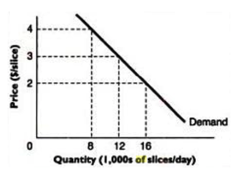
However, the quantity consumed is affected by the prevailing market price. This is illustrated by figure 1 (Bernanke 2004, p. 61).

A fundamental property of the demand curve is that it is downward sloping with respect to price. As can be seen from figure 1, it is clear that consumers will purchase more when prices are low and vice versa.
Obviously, the demand curve can be interpreted either vertically or horizontally. Under the horizontal interpretation, we begin with a price and then end up with the quantity demanded at that price.
For example, at a price of $ 4 only 8,000 units will be demanded per day while at a price of $ 2, consumers will demand up to 16,000 units. Under the vertical interpretation, we begin with a quantity a specific quantity and go on to determine the price from the demand curve.
For example, when the demand is high, at 16,000 units per day, a lower price of $ 2 is charged while when the supply is only 8,000 units per day, a higher price of $ 4 is charged.
Supply
As stated earlier, a high supply of a good or service will result in lower prices while a decline in supply will lead to higher prices. Although some shortages in supply may be natural, others may be influenced by sellers who are out to extort money from unsuspecting consumers (Myers 2004, p. 23).
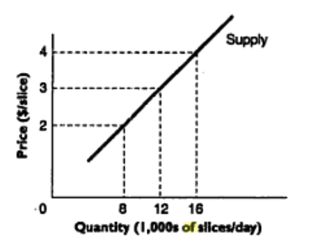
Clearly, when the supply is low, a higher number of consumers will be fighting to get the same commodity. If this happens in a free market economy, the consumer becomes the biggest loser. Figure 2 illustrates how supply affects prices.

Like the demand curve, the supply curve can be interpreted either horizontally or vertically. Under the horizontal interpretation, we being with a price and then go over to the supply curve to check the quantity that sellers wish to sell at that price on the horizontal axis.
For example, at a price of $ 2, sellers are willing to sell 8,000 units in a day. Under the vertical interpretation, we begin with a quantity and then determine the corresponding price from the supply curve. For example, when the quantity supplied is 12,000 units, the corresponding price is $ 3.
Equilibrium Price and Equilibrium Quantity
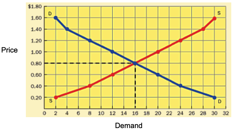
The equilibrium price is that price that sets buyers’ plans equal to sellers’ plans. Similarly, the quantity at which these plans are equal is referred to as the equilibrium quantity. Therefore, in a free market economy, the equilibrium price and quantity are the price and quantity toward which markets will automatically move.
At the equilibrium price, the quantity demanded equals the quantity supplied and neither sellers nor buyers will want to change the price or the quantity (Welch & Welch, 2009).
Often, the equilibrium price is referred to as the market clearing price since at this price, the amount buyers want exactly matches the amount that sellers offer, thereby clearing the market of the good or service.
When the price of a good or service is below its equilibrium level, a shortage will develop, and the price will be driven up toward the equilibrium. On the other hand, if the price is above the equilibrium, a surplus will develop, causing the price to fall toward equilibrium.
Figure 3 a combined graph of demand and supply curves and illustrates the equilibrium price and equilibrium quantity (Welch & Welch, 2009).

Factors that have Led to the Rises in the Prices of Cereals in the Past Five Years
As noted by Meyer (2012, p. 1), poor weather conditions played a big role in the rise of prices of cereals in the past five years. To a great extent, this is also related to the devastating effects of global warming and climate change.
Although other factors are partly to blame for the pathetic weather experienced in most parts of the world, increased activities on earth by men and women are largely responsible for degrading the environment. The result of this has been severe droughts in any countries and hence poor harvests.
The poor harvests automatically imply that the quantity of cereals supplied can not meet the market demand. Clearly, the low supply and high demand imply that the prices of cereals had to go up.
A study by the World Bank also arrived at the conclusion that weather is the most critical factor that is to blame for the soaring prices of cereals (World Bank, 2012, p. 2). The unfavorable weather is generally blamed for vast damage caused to cereal crops and hence affecting the output from farms.
As noted by Odland (2012, p. 1), restrictions by the government are also to blame for the rise in cereal prices. Even though this may be beneficial to some degree, it can easily lead to poor harvests. Increased prices are also linked to the fact that the rise in the cost of oil directly affects the cost of transport as well as other production materials.
In places like China and India, where the population is always on the rise, a high demand for food stuff leads to high prices for goods and services.
Another factor that has led to the rise in prices of cereals is absence of government subsidy (FAO 2011, p. 13). Among the most important forms of government assistance to farmers is the fertilizer subsidy. Where fertilizer subsidies are provided by the government, commodity prices tend to be lower.
Since farmers receive fertilizers at reduced prices, they are also able to sell their produce at lower prices without going into a loss. In the past five years, however, changes in government policies touching on subsidies for cereal crops have led to increased prices (OECD 2008, p. 8).
Unfortunately, the government of the United States has been accused of encouraging farmers to engage in farming practices that consume little water.
In as much as this may be of some benefit to the environment, it has the negative repercussion of reducing food supply. The decline in food supply in turn leads to low supply and this eventually results in high commodity prices.
Reference List
Bernanke, B. 2004, Principles of Microeconomics, The McGraw-Hill Companies, Inc., Hong Kong, China.
Food and Agricultural Organization (FAO), 2011, Recent Trends in World Food Commodity Prices: Costs and Benefits. Web.
Grant, S. & Vidler, C. 2000, Economics in Context, Heinemann Educational Publishers, Sandton.
Jones, T. 2004, Business Economics and Managerial Decision Making, John Wiley & Sons, Hoboken, NJ.
Mankiw, N. G. & Taylor, M. P. 2006, Microeconomics, Cengage Learning EMEA, Bedford Row, London.
Meyer, G. 2012, Moment of Truth for US Grain. Web.
Mukherjee, S. 2007, Modern Economic Theory, New Age International, New Delhi, India.
Myers, D. 2004, Construction Economics: A New Approach, Taylor & Francis, New York, NY.
Odland, S. 2012, Why Are Food Prices So High? Web.
Organization for Economic Co-operation and Development (OECD), Rising Food Prices: Causes and Consequences. Web.
Welch, P. J. & Welch, G. F. 2009, Economics: Theory and Practice, John Wiley & Sons, Hoboken, N. J.
World Bank, 2012, Poverty Reduction and Equity Group Poverty Reduction and Economic Management (PREM) Network. Web.