The impact of factors on GDP and each of its components and the level of unemployment
Keynesian 45° model of economic variable comparison was derived by compares aggregate expenditure (C+I+G+X-M) and National Income in an economy and suggested that at an optimal state, where an economy has no surplus or deficit, then the relationship between the two forms a 45° angle curve; the following curve represents the model:
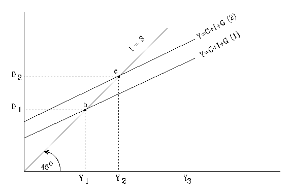
A brief analysis of the diagram: the above 45° diagram is the version of the Keynesian model, the line making 45° is the line where the AE aggregate Expenditure (C+I+G+X-M) = National Income Y, this can only be attained an idea economic situation which is hard to come by.
This paper interpolates the effects on the following:
An increase in the domestic rate of interest
When the rate of interest is increased, then the cost of getting finances is increased, the most direct result is a reduction in investments, investment results to reduce the consumption reduces since the people have no source of spending money.
Investments are the exporters, when they have been reduced, then the economy suffers reduced exportation; people will opt to buy imported goods since the cost of producing local goods has increased and with a reduced number of investments. The net result is increased importation.
The GDP reduces and there will be an increase in the unemployment level in the economy. When an economy has a high rate of unemployment, then government expenditure will increase.
A decline in consumer confidence
When consumers do not have confidence with goods produced in the economy; then they are likely to buy imported goods which they believe are of better quality, importation thus increases. The economy will have reduced demand for goods locally thus local consumption will reduce: firms will have reduced businesses thus they will not be willing to invest further in the economy, thus investments reduce. When the local economy is not expanding, then the economy is not producing commodities to export, the exportation reduces.
In the situation, the economy is not expanding thus employment rate will reduce or the unemployment rate will be increased, as well as the GDP of a country. When an economy has a high rate of unemployment, then government expenditure will increase.
A decrease in the general rate of taxation
The decrease in taxation, holding other economic factors constant, affects investments, people will be willing to invest in the economy since they will enjoy a low rate of taxation; with an economy with increasing investments, then the rate of unemployment will be reduced and the consumption of the economy increased.
An economy with investments is a growing economy thus the economy will be on an upward rise. The investments will be increased thus increasing consumer goods leading to a decrease in importations. Firms will have good o export thus the country will enjoy a higher rate of exportation.
When the economy is expanding and leading to more capitalism, government expenditure is reduced unless it is used for expanding infrastructures in the economy to facilitate further trade.
An increase in government expenditures
Government expenditure in an economy is expected to attract investments when there is a high budget in improving infrastructures, thus an increase in government expenditure means an increase in investments. A country that is having increased investments is likely to increase the number of locally produced goods thus; there will be an increase in consumption. Investments, on the other hand, come with increased employment chances thus the economy will have a reduced unemployment rate. A county will high employment and increased domestic consumption has a high rate of GDP growth. Firms established to enjoy the benefits likely to be accrued from increased government budget results in an increase in consumer goods thus importation will reduce.
An increase in the exchange rate (the home currency increases in value)
When the home currency gains value, then importation becomes expensive, when goods become expensive them there is a shift to another alternative. The increased cost of importation results in a decrease in importation thus the domestic product consumption will be increased. When a currency is valued, then exportation becomes cheap and attractive, exporters get a higher return so they will be willing to export, exportation increases. With the increase in international trade, firms are willing to invest in areas that there are low export costs and those that concentrate on local consumption, in the result is an increase in investments. A country that can sustain its population through employment has minimal government expenditure.
A boost in investment results in an increase in employment and the GDP of the country increases.
An increase in the price of Brent crude
Fuel is an important element in the production of goods and services, when the cost of fuel increases, then a country suffers an increased cost of production; thus investments decrease. A decrease in investment means an increase in unemployment and increased government expenditure, and the rate of domestic consumption is reduced. Importation and exportation are elements determined by investment, when the rate of investment is reduced like it is in the case, then the exportation reduces and importation increases.
“Aggregate Supply” curve derived under Keynesian and “classical” scenarios
Keynesian
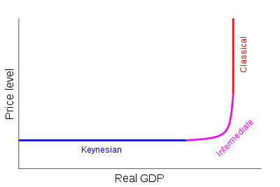
Aggregate supply refers to the total expected sales in an economy over a certain duration: when drawn it represents a comparison between real production and the price level. Keynesian aggregate supply curve has segments: one segment is rather horizontal indicating that along the line prices are rigid resulting in reduced real production, the second segment is rather vertical. The vertical side represents full employment which results from limited production and fixed total quantities of resources. The curve looks
Classical
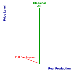
The main point of Classical theorists is that an economy has the mandate and capability to maintain a full-employment level, which creates a vertical supply chain line; the line implies perfectly inelasticity. The curve resembles a long-run supply curve:
It looks like:
Comparison of the supply and demand curves of microeconomics and their aggregate counterparts
Supply and demand curves
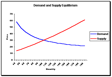
The diagram below shows supply and demand curves: the curve is derived from a comparison of individual firms, industry, or consumer quality consumed at different prices. At the equilibrium, then demand = supply. At any point above the equilibrium, then the prices are high that suppliers are willing to supply more than demand, the market then has a surplus, below the equilibrium, then the prices are not encouraging for suppliers to supply commodities, the market suffers a deficit.
Aggregate Supply and Aggregate Demand curves
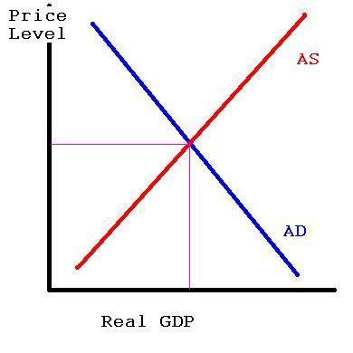
The diagram below show a hypothetical AS and AG curve: it has the price in the economy at the Y-axis and Real GDP as the X-axis, at equilibrium, the economy is said to be producing at an optimal rate where there is no excess or deficit: this is an assumption that cannot be attained.
Differences
Similarities
Both supply and demand curves of microeconomics and their Aggregate Supply and Aggregate Demand curves equilibrium is affected by similar factors. A factor that is likely to cause an upward rise in either curve causes a similar effect on the other curve. For example, a change in prices of goods upwards will have a similar effect on both curves.
In both curves, they have prices of commodities in the Y-axis and the slope of the graphs defines the relationship between prices and aggregate supply or aggregate demand. The idea is the same but developed at different stages; they also have quantity variable on the X-axis and use the two to analyze the economic situation though at different levels.
Both the graphs assume that an optimal level, where there is no surplus or deficit, exists, this can only happen at an ideal economy.
References
Roger A. Arnold. 2008. Macroeconomics. Gale: Cengage Learning.
Snowdon, Howard. 2005. Modern macroeconomics: its origins, development, and current state. Massachusetts: Edward Elgar Publishing.